13. Object Detection

This Object Detection is of three types

1. Object Classification - In this we give a name to the image. e.g.: A Car
2. Image Localization - In this we locate the instance of an object category in the Image, Showing the Image using a bounding box. e.g.: Rounding of the car using a box in the Image
3. Object Detection - In this we locate all instances of all the classes inside the Image. This classification comes from a predefined set of categories in the dataset. e.g.: A bunch of cars and the Mountain behind it, all should be rounded in a bounding box

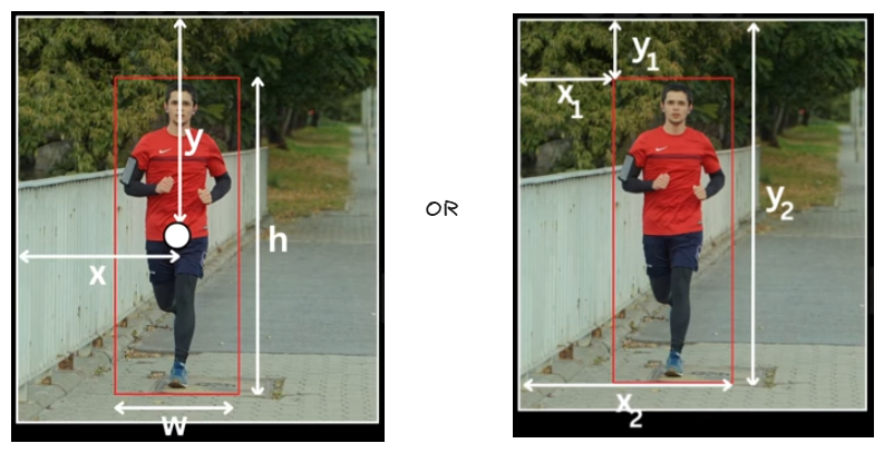
Our task is to design a model which draws the bounding box(a square/rectangle box indicating a feature/object) for the given Image and does Object Detection The bounding box can be any of this two, and the arrows show the co-ordinates

Approach 1: CNN

• Get the input image and draw all the possible squares/rectangles in that image and pass it to convolution and pooling layers, this will extract all the features from previous layers and have them as flatten tensors, from here we have two branches to calculate loss
  1. These Tensors are passed to a fully connected classifier(4096 to 1000) at the end that will give the scores for each possible object and these are compared with correct label by passing through Supervised Learning Classifier, that gives us the Cross Entropy Loss
  2. The same Tensors are also passed to a fully connected classifier(4096 to 4) at the end they will give us bounding box co-ordinates, these are compared with correct box labels by passing through Supervised Learning Classifier, this gives us L2 Loss
• Cross Entropy Loss + L2 Loss = Total Loss
• But this approach can only detect one object like if we give an image with multiple cars, it can only detect one car, this process of having ability to detect only one is called Object Localization

$$\sum _{h=1}^H\sum _{w=1}^W(W-w+1)(H-h+1)=\frac{H(H+1)W(W+1)}{4}$$

• Also it takes around(above formula) operations to get the result
  • W, H - width and height of the Input Image
  • w, h - width and height of the bounding box

Approach 2: R-CNN

This R-CNN is of 6 steps

1. Extract Region Proposals using Selective Search
   • Rather exploring every possible bounding box in the given input image, we can use a external algorithm called Selective Search to narrow down the possible bounding boxes called region proposals(~around 2000 images), these region proposals are filtered if they have proposal overlap > 50%(IOU >= 0.5) if they do, then transformed into a square(227x227 for AlexNet compatibility) with co-ordinates (px, py, ph, pw) and dilate(zooming out in the same size) the bounding box, such that it have p pixels(p=16) as context, if the image is already fit, we add some padding and then dilute to get that p=16 value, and this completes our dataset
2. Train AlexNet(or VGGNet which gives higher accuracy but takes more time), on ImageNet Classification Dataset
   • To Perform feature extraction we need a classifier, so we train a large Convolution network called AlexNet
   • After this we remove the last classification layer and now we add a new classification layer which caters to classes present in our detection dataset
   • Now if we have two classes to detect, e.g.: Person and Car (say n classes), then our classifier layer will have three output layers (n+1), two for classes and one in background
3. Fine tune CNN with resized proposals on classes of detection dataset and background class
   • Here we divide the data into two batches
     1. Image which have ground truth(human labelled, correct bounding boxes) bounding boxes
     2. Image with region proposal(~2000 bounding boxes)
   • Using these two batches we fine tune our Network work on categories present in our detection dataset plus the background task and train the whole network using cross-entropy loss, After fine tuning we remove the classification layer and use Fully Connected Layer output as feature representation of the proposals

Q What if we have two ground truth boxes by which a proposal overlaps. e.g.: A Dog in the laps of a human, here what do we label the bounding box as a human or a dog ?
A We consider the ground truth box that has higher overlap with the proposal, so in this as the human is big, we label it as a human

4. Train Binary Classifier(SVM) for each class and on fully connected layer representation of proposals
   • SVM(Supervised Machine Learning) is a linear classifier which learns a decision boundary in 4096 dimensional space, so the person class SVM is going to learn to use this features to classify the proposals as Person or not a Person
   • Now we train a Linear SVM for each class which takes this feature representation and learns to classify whether it’s a positive instance or a negative Instance of the Class
   • Here we have a ground truth label, which we take as reference to label a input as positive or negative
     • Positive labelled proposals for class K → Ground truth Box
     • Negative labelled proposals for class K → Proposal boxes < 0.3 IOU with all instances of that class

Q As we have a fine tuned model in the 3rd step, why we need SVM then ? or As we have SVM which classifies each class on fc layer representation of proposals in 4th step, why we need Fine tuned CNN in the 3rd step ?
A They both act as two layers of filters

• Fine tuned CNN - gives multiple bounding boxes for the target, avoids overfitting
• SVM - act as a Boolean filter for the boxes coming from fine tuned model

5. Train a class specific Bounding Box Regressor on top of proposal features

   • We’re currently relying on the regional proposals coming from Selective Search algorithm, but there is a problem with it

     • Proposal slightly misses left edge of subject → box prediction will be inaccurate
     • Proposal too large around person → includes extra background
     • Proposal with wrong aspect ratio → box needs adjustment

   • Input: Proposal box P with coordinates (px, py, pw, ph) where (px, py) = center, (pw, ph) = width/height Target: Ground truth box G with coordinates (gx, gy, gw, gh) Learn: Transformation T such that T(P) ≈ G

     T defined by parameters: (tx, ty, tw, th) Transformation:

     • gx ≈ px + pw . tx
     • gy ≈ py + ph . ty
     • gw ≈ pw . exp(tw)
     • gh ≈ ph . exp(th)
6. Filter prediction using NMS (Non-Maximum Suppression)
   • After all previous steps, for a single object, we might have:
     • Multiple proposals (from Selective Search) hitting same object
     • Each proposal refined by bounding box regressor
     • Each passed SVM classification
   • This leads to Multiple overlapping boxes for same object instance for example:
     • Person in image gets predicted as:
       • Box 1: (150, 200, 100, 150) - confidence 0.95
       • Box 2: (153, 202, 102, 148) - confidence 0.92
       • Box 3: (155, 205, 98, 145) - confidence 0.88
       • Box 4: (200, 300, 100, 150) - person wearing hat (different person, low confidence)
       • Box 5: (230, 290, 95, 140) - hat area (very low confidence)
   • To solve this problem, we follow the NMS Algorithm

• NMS is a post-processing technique that eliminates duplicate and overlapping bounding boxes, selecting only the most confident and relevant boxes corresponding to detected objects
• The algorithm operates by iterating through predicted bounding boxes and uses two key metrics: confidence scores and an Intersection over Union (IOU) threshold
• If two bounding boxes have an IOU overlap exceeding the defined threshold (typically 0.5), they are considered duplicates pointing to the same object
• NMS keeps the box with the highest confidence score and suppresses (removes) all other overlapping boxes that have IOU greater than the threshold
• If overlapping bounding boxes point to different objects, they are both retained since they represent distinct detections
• The IOU threshold is a user-defined hyperparameter: a lower threshold results in fewer detections by suppressing more boxes, while a higher threshold may allow multiple detections for the same object
• Mean Average Precision (mAP) is an evaluation metric used to assess overall model performance after detection and post-processing are complete. The mAP is then the average of these Average Precision (AP) values across all classes. The IOU metric is used within mAP calculations to determine whether a predicted box is considered a true positive or false positive​
• At Last we have a model, which had trained to predict the a given class objects in the given Input Image

Approach 3: Fast R-CNN

It’s simply making the R-CNN faster, there are three places we can optimize it

1. Object detection is Slow

• There is a problem of slow inference because at test time, features are extracted from each object proposal in each test image, that means the detection with VGG16 takes 47sec/image (on Nvidia k40 GPU ~ Older GPU)
• Let’s optimize it, Here we know that we do forward pass through the CNN for all the proposals for a given image, because we need feature representation for each proposal for later prediction layers. Instead of running the CNN separately on every proposal, we can run the CNN once on the entire image and then crop the proposal regions directly from the final feature map. However, these cropped regions have different spatial sizes, and flattening them produces feature vectors of varying dimensions, but we have a problem here, we cannot fed this into fully connected layers because they expect a fixed-size input
• ROI Pooling solves this by taking each proposal’s feature-map region and converting it into a fixed-size output (e.g., 7×7). This ensures every proposal produces a uniform-length vector after flattening, allowing consistent input to the FC layers

2. Training is Multi Stage Pipeline

• Rather than one training task, to train R-CNN we need to manage the entire pipeline of three sequential training tasks(fine tune CNN, SVM, bounding box regression)
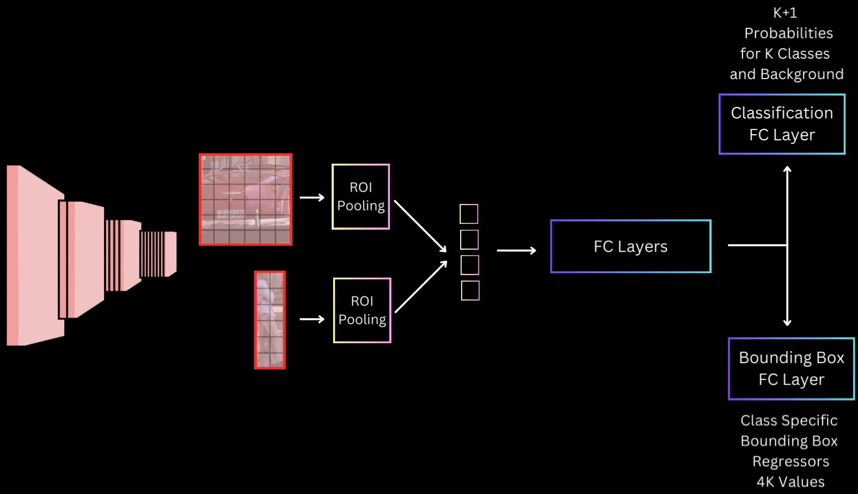
• Let’s optimize it, Rather than having 3 stages of training as an R-CNN, we take the flattened ROI pooling output, feed it to a few common Fully Connected Layers and then have two branches of Fully connected layers
  1. Classification FC Layer - Responsible for predicting the class probabilities for the proposal for the K + 1 Classes including Background
  2. Bounding Box FC Layer - It predicts 4K values, which are the four regression values for the K classes

3. Training is Expensive in Space and Time

• For SVM and bounding box regressor training, features are extracted from each object proposal in each image(~2k region proposals) and written to disk

Implementation Details

Quantization and Coordinate Alignment Issues:
When mapping an ROI from image space to feature map space, we encounter a issue wrt non-integer boundaries
Setup:

• Image size: 400 × 400
• CNN stride: 40 → feature map becomes 10 × 10
• ROI (image space):

$$(x_{\text{img}},y_{\text{img}},w,h)=(10,;20,;50,;60)$$

Mapping to feature map:

$$x_{\text{feat}}=\frac{x_{\text{img}}}{S}=\frac{10}{40}=0.25$$

Feature maps require integer indexing, so we quantize:

$$x_{\text{feat}}=\lfloor 0.25\rfloor =0$$

Misalignment introduced:

• Some true ROI pixels get excluded
• Some outside pixels get incorrectly included

This is an acceptable approximation in Fast R-CNN

Bin Division Using Floor/Ceil: For an ROI of size:

$$(h_{\text{roi}},w_{\text{roi}})$$

divided into a grid:

$$(h_{\text{pool}},w_{\text{pool}})$$

bin boundaries:

$$h_{\text{start}}(j)=\lfloor j\cdot \frac{h_{\text{roi}}}{h_{\text{pool}}}\rfloor$$ $$h_{\text{end}}(j)=\lceil (j+1)\cdot \frac{h_{\text{roi}}}{h_{\text{pool}}}\rceil$$

Similarly:

$$w_{\text{start}}(i)=\lfloor i\cdot \frac{w_{\text{roi}}}{w_{\text{pool}}}\rfloor$$ $$w_{\text{end}}(i)=\lceil (i+1)\cdot \frac{w_{\text{roi}}}{w_{\text{pool}}}\rceil$$

Example (8×7 ROI → 2×2 bins):

• Bin height: $\frac{8}{2}=4$
• Bin width: $\frac{7}{2}=3.5$ For bin (1,1):

$$h_{\text{start}}=\lfloor 1\cdot 4\rfloor =4,h_{\text{end}}=\lceil 2\cdot 4\rceil =8$$ $$w_{\text{start}}=\lfloor 1\cdot 3.5\rfloor =3,w_{\text{end}}=\lceil 2\cdot 3.5\rceil =7$$

for c in range(C):
    for j in range(h_pool):
        for i in range(w_pool):
 
            h_start = floor(j * bin_size_h)
            h_end   = ceil((j+1) * bin_size_h)
            w_start = floor(i * bin_size_w)
            w_end   = ceil((i+1) * bin_size_w)
 
            region = roi_features[c, h_start:h_end, w_start:w_end]
            output[c, j, i] = max(region)

Transition to FC Layers & Output Heads

Flattening:
ROI pooled feature map (VGG-16):

$$7\times 7\times 512=25088$$

FC6 / FC7 Architecture:

$$25088\to 4096\to 4096$$

Pretrained on ImageNet → reused here
Classification Head:

$$4096\to (K+1)$$

Output SoftMax:

$$p=(p_0,p_1,\dots ,p_K)$$

Bounding Box Regression Head:

$$4096\to (4K)$$

Transforms:

$$x^{\prime }=x+t_x^{(u)}w$$ $$y^{\prime }=y+t_y^{(u)}h$$ $$w^{\prime }=w\cdot e^{t_w^{(u)}}$$ $$h^{\prime }=h\cdot e^{t_h^{(u)}}$$

Multitask Loss (Joint Classification + Localization)

Full Loss: $$
\mathcal{L}(p, u, t^u, v)

\mathcal{L}{\text{cls}}(p, u)
+
\lambda \cdot [u \ge 1] \cdot \mathcal{L}{\text{loc}}(t^u, v)

\mathcal{L}_{\text{cls}}(p, u) = -\log p_u

$$RegressionLoss(SmoothL1):$$

\mathcal{L}{\text{loc}}=\sum{i\in{x,y,w,h}} \text{SmoothL1}(t_i^{(u)} - v_i)

$$SmoothL1:$$

\text{SmoothL1}(\Delta)=
\begin{cases}
0.5\Delta^2 & |\Delta| < 1 \
|\Delta| - 0.5 & \text{otherwise}
\end{cases}

$$Regressiononlyforforeground:$$

[u \ge 1]

##### Pretrained Initialization #Q Why ImageNet Pretraining? #A Generalizable low-level features → faster training, higher accuracy Changes to be made: - Replace final max-pool → ROI Pooling - Keep FC6, FC7 - Remove ImageNet classifier - Add detection heads (classification + bounding box) Weight Initialization: - Conv + FC6, FC7 → pretrained - Heads → random small Gaussian ##### Sampling & Mini-batches Batch Structure Example: - Images per batch: `N = 2` - Proposals per batch: `R = 64` IOU-Based Proposal Assignment - Foreground: `IOU > 0.5` - Background (hard negatives): `0.1 <= IOU <= 0.5` - Ignored: `IOU < 0.1` 25% Foreground Sampling Rule

\frac{FG}{Total} = 0.25

For 64 proposals: 16 FG and 48 BG (hard negatives) ##### Scale Invariance A CNN trained on 224×224 ImageNet images sees objects at a canonical size. In the real world, the same car appears at vastly different pixel sizes: - Close to camera: 400×300 pixels - 10 meters away: 150×100 pixels - 50 meters away: 40×30 pixels If the network only learned one scale, it would fail on distant objects. Scale invariance means the detector performs equally well regardless of object size _Approach 1: Brute-Force Single-Scale_: How it works: - Resize every training and test image to a fixed size, e.g., 600×600 - Train the network on this canonical size - During inference, all images are resized to 600×600 before detection - The network implicitly learns scale invariance from the data distribution (large objects in the dataset get squashed, small ones get enlarged) Limitations: - Distorts aspect ratios (a 1920×1080 image becomes 1:1 square) - Small objects are down sampled further; large objects clipped - Some information loss due to nonuniform scaling _Approach 2: Multi-Scale Image Pyramid_: Core idea: Process each proposal at the scale where it appears closest to its natural 224×224 size (ImageNet standard) 1. Building the Pyramid Create an image pyramid at multiple scales:

\text{Pyramid Scales} = {1.0,; 0.75,; 0.5,; 0.25} \times \text{original image size}

$$Foran800\times 600image:-Scale1.0:800\times 600-Scale0.75:600\times 450-Scale0.5:400\times 300-Scale0.25:200\times 1502.Proposal-to-ScaleAssignmentForeachproposal,computeitsareaateachscaleandassigntothescalewheretheareaisclosestto:$$

224^2 = 50{,}176

Example proposal Width = 320, Height = 240 → Area = 76,800 | Scale | New Size | Area | Distance to (224^2) | | ----- | -------- | ------ | ------------------- | | 1.0 | 320×240 | 76,800 | 26,624 | | 0.75 | 240×180 | 43,200 | 7,776 | | 0.5 | 200×150 | 30,000 | 17,024 | | 0.25 | 80×60 | 4,800 | 45,376 | 3. Feature Extraction per Scale - Compute backbone features for each pyramid scale - For each proposal assigned to scale (S): - Extract ROI pooled features from that scale’s feature map. - Pass through shared FC layers + heads Advantages: - Small objects get upscaled → details preserved - Large objects get downscaled → fit without clipping - All proposals are processed near the canonical ImageNet resolution 4. Inference Procedure (Multi-Scale) ```python for each image: create pyramid (scales: 1.0, 0.75, 0.5, 0.25) for each scale in pyramid: compute backbone features run Selective Search on this scaled image for each proposal: compute its area find scale closest to 224^2 extract RoI pooled features from that scale classify + regress combine predictions from all scales apply NMS per class ``` _Summary_: | Aspect | Single-Scale | Multi-Scale | | -------------- | -------------------------------------------- | ------------------------------------------------------------------------- | | What it does | Resizes all images to 600×600 | Creates image pyramid; assigns each proposal to scale where it's ~224×224 | | Speed | Baseline (1 backbone pass) | +14% slower (4 backbone passes) | | Accuracy | 66.9% mAP | 67.4% mAP (+0.5% gain) | | Why chosen | Speed/accuracy trade-off favors single-scale | Complexity + slowdown not justified | | Real-world use | All production systems | Research/academia only | | Future | Replaced by FPN-based methods | Replaced by FPN-based methods | #### Approach 4: _Faster R-CNN_ Same as before, we optimize the layers to make the R-CNN faster. Here the Selective Search Step is slow, thus we replace that with a CNN module called [[13. Object Detection#rpnregion-proposal-network|RPN (Region Proposal Network)]], this RPN will return the regions which possibly contain an object(same functionality of selective search) and pass this RPN generated regions to ROI pooling 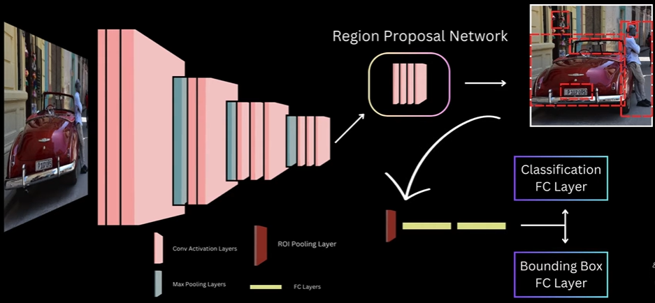![[Pasted image 20251119164718.png]] #### Approach 5: _YOLO V1_ There are two kinds of object detection models 1. One Stage, where we detect object class stores and detect the object boxes in one pass 2. Two Stage, where the above two happens in two steps Here we pass the input Image to a YOLO CNN Model and this outputs the multiple bounding boxes and probabilities for those boxes. And here is the step by step implementation of YOLO CNN Model 1. Divide image into `S x S` grid cells 2. Each target object is assigned to the cell that contains the objects center 3. Each grid cell predicts B bounding boxes 4. YOLO is trained to have box predictions of each cell as close as possible to the target assigned to the cell. And it follows below steps to predict the box - With respect to x offset and y offset we calculate the center of the image, if the image offset is 0, then the center will be in the top, if it's 1 then it will be below, with respect to center we take out the box - We also calculate how confident the model is to say that the object is in the predicted box. Thus we calculate "how accurate or good fit the predicted box is for the object it contains" - For each bounding box we will have 5 prediction values(x, y, w, h, conf) and along with this YOLO also predicts the class conditional probabilities. Thus at last we predict _(5 x B) + C_ values, where B is number of bounding boxes and C is the classes(which are of same number of ground classes) - Here for each grid cell, YOLO predicts one set of class probabilities, It means it can't predict multiple objects from single bounding box, if we want to predict multiple objects we need to run multiple networks to one for each object - YOLO will predict multiple boxes(B>1) per grid cell, but only one predictor box is responsible for that target, the one with highest IOU with the target box _YOLO Architecture_: - Given an Image the CNN used by authors generates a output with _S x S x ((5 x B) + C))_ for the entire image, this will entirely transform _S X S_ grid with _(5 x B)+ C_ channels for all the grid cells of input Image - For example if we take a 3 x 3 grid cells, the number of boxes per grid cell is 2 and number of classes is 20, this CNN will return prediction values that can be transformed into a 3 x 3 grid output with 30 channels and each output cell will represent the prediction values for that grid cell ![[Pasted image 20251203210518.png]] - For the Model, authors used Google Net network, but instead of the inception modules, they replaced it with `1 x 1` and `3 x 3` convolution layers, they first trained this network on image net classification task, by stacking FC layers and training on image sizes of 2224 x 224, post that they get rid of the FC layers and add additional convolution layers prior to detection training specifically 4 convolution layers, after these convolution layers we have two FC layers to find predict our `S x S x ((5 x B) + C)` dimensional tensor of prediction values which can be reshaped to create out S x S grid outputs. Here is the Final Architecture ![[Pasted image 20251203211101.png]] _YOLO Loss_: ![[Pasted image 20251203221812.png]] - In YOLO any target object is only assigned to one grid cell, the one which contains the center of the object and out of all the predictor boxes, only one is responsible for the target, the one which has the highest IOU with ground truth - There are three types of Loss in this 1. Localization Loss - The model learns to predict the XY offset and width and height prediction values of the responsible predictor box of a cell closer to the target assigned to that cell

\lambda_{coord} \sum_{i=0}^{S^2} \sum_{j=0}^{B} \mathbb{1}^{obj}_{ij} \left[(x_i - \hat{x}_i)^2 + (y_i - \hat{y}_i)^2 \right]

$$-Penalizeserrorinpredictedboxcentercoordinates.Onlyappliedwhenaboxcontainsanobject$$

\lambda_{coord} \sum_{i=0}^{S^2} \sum_{j=0}^{B} \mathbb{1}^{obj}_{ij} \left[(\sqrt{w_i} - \sqrt{\hat{w}_i})^2 + (\sqrt{h_i} - \sqrt{\hat{h}_i})^2 \right]

$$-Penalizeserrorinpredictedwidthandheight.Squarerootsreducetheimpactoflargeboxsizes.Alsoappliedonlyforobject-containingboxes,I{t}^{\prime }smultipliedbylambdawhichincreasedthevalueofthelocalizationaccuracy2.ConfidenceLoss-Thisismeanttotrainthemodeltocapturetwoaspects,whicharetopresenceofanobjectandaswellashowgoodfitthepredictedboxis.SowewantthehighvaluewithoverlapwiththegroundtruthtargetandlowervaluewhentheboxcontainsandobjectbutdoesnotfitwellandZerowhenthereisnoobject,thereforetrainingthemodelattesttime,wheretherewillbenogroundtruthavailable$$

\sum_{i=0}^{S^2} \sum_{j=0}^{B} \mathbb{1}^{obj}_{ij} (C_i - \hat{C}_i)

$$-Penalizesconfidencescoreerrorsforboxesthatcontainanobject-Ci:ground-truthconfidence=1-C{i}^{}:predictedconfidence(IoU-based)$$

\lambda_{noobj} \sum_{i=0}^{S^2} \sum_{j=0}^{B} \mathbb{1}^{noobj}_{ij} (C_i - \hat{C}_i)

$$-Penalizesconfidenceerrorforboxeswithoutobjects-I{t}^{\prime }smultipliedbylambdatoreducetheimpactofoverwhelmingnegativesamples,typicalvalueis\mathrm{0.53.}ClassificationLoss-Thiscontainsthemodelthatshouldpredict‘one‘asthevalueforthatclassand‘zero‘fortheremainingclasses$$

\sum_{i=0}^{S^2} \mathbb{1}^{obj}{i} \sum{c \in classes} (p_i(c) - \hat{p}_i(c))

- Penalizes error in predicted class probabilities. Applied only to cells that contain objects - pi(c): ground-truth one-hot class label - pi^(c): predicted probability - And at last we will train the detection network on resized images of 448x448 - Code Implementation: [GitHub](https://github.com/explainingai-code/Yolov1-PyTorch) #### Approach 6: _SSD (Single Shot Multibox Detector_ This is also a one stage object detector, like YOLO V1. It means here we have single model which will be detecting all the bounding boxes and there class probabilities for a class present in an Image Here the bounding boxes implementation is nearly same as in [[13. Object Detection#approach-4-_faster-r-cnn_|Faster R-CNN]] where it uses [[13. Object Detection#rpnregion-proposal-network|RPN]], in which we have a backbone which is VGG16 implementation and using the last convolution layers feature map, we made predictions for the set of preference boxes of specific scales and aspect ratios, centered at the center of each of the feature map grid cells and using 3x3 convolution kernel we predicted transformation parameters to transform reference boxes to tightly fit the underlying object SSD almost works the same but with following differences 1. Rather than just, predicting the probability that the reference or default box contains an object or not, we predict the probability score for all categories present in our dataset, including background 2. We don't just make predictions for default boxes on the last feature map but in fact use feature maps of multiple layers at different resolutions and make predictions for default boxes of different scales and aspect ratios for each of these feature Maps - During training given an image and ground truth SSD decides which of these default boxes should be treated as a background box and learns to classify those as background class and which should be matched to a ground truth object - The raw feature maps are directly used this aspect of using feature maps from different stages of Network to make predictions for default boxes of different scale earlier layers used for small scale default boxes and later layer outputs used for large scale default boxes this was the key contribution of SSD and it allows us to get higher accuracy while using a relatively lower resolution input than YOLO V1 and because of using lower resolution input we also see an increase in detection speed a aside from this the authors also use hard negative mining to select difficult negative examples during training and extensive data augmentation to make the detector robust _Default Boxes_: SSD relies on predictions from multiple feature maps, each operating at a different spatial resolution. The original SSD model uses modified VGG-16, but the backbone is not crucial; what matters is that it produces six feature maps with sizes: 38×38, 19×19, 10×10, 5×5, 3×3, 1×1. These multi-resolution maps allow SSD to detect objects of varying scales: high-resolution feature maps detect small objects, while low-resolution feature maps detect large objects - Each feature map is assigned a single scale value. SSD computes these scales using a simple linear interpolation between a minimum scale(s_min = 0.2) and a maximum scale(s_max = 0.9), across the total number of feature maps (m) The scale for feature map ( k ) is:

s_k = s_{\min} + \frac{s_{\max} - s_{\min}}{m - 1}(k - 1)

$$-Thisensuresthatthefirstfeaturemapusessmallanchorboxes(scale0.2)andthelastuseslargeones(scale0.9),withintermediatemapsreceivingevenlyspacedscales.Forexample,with5featuremaps,thescalessmoothlyprogressfrom0.2\to 0.9,coveringtheentirerangeofobjectsizesinanimageForeachscale(s_k),SSDdefinesmultipleaspectratios,typically:$$

a_r \in {1, 2, \frac{1}{2}, 3, \frac{1}{3}}

$$Givenscale(s_k)andaspectratio(a_r),thewidthandheightofthedefaultboxarecomputedas:$$

w = s_k \sqrt{a_r}

h = \frac{s_k}{\sqrt{a_r}}

$$Theseformulaskeeptheareaoftheboxconstantsince:$$

w \cdot h = s_k

$$Thisguaranteesconsistentcoveragewhilechangingonlytheshapeofthebo{x}_{E}xtraBoxforAspectRatio=1_{:}Toimprovecoverageforintermediatescales(especiallybetweentwofeaturemaps),SSDaddsaspecialadditionalboxwithaspectratio1butwithageometricmeanscale:$$

s’k = \sqrt{s_k \cdot s{k+1}}

$$Thisextraboxensuressmoothertransitionsbetweenobjectsizesandreducesdetectiongapsbetweenadjacentscale{s}_{D}efaultBoxCenter{s}_{:}Eachfeaturemapcellcorrespondstoagridlocationintheimage.Forafeaturemapofspatialdimension‘FxF‘,thecenterofthecellatindex(i,j)iscomputedby:$$

c_x = \frac{j + 0.5}{F} , c_y = \frac{i + 0.5}{F}

$$Thesecoordinatesarenormalizedtolieintherange(0,1).Thus,regardlessofimagesize,thedefaultboxesalignperfectlywiththegridstructurederivedfromthebackboneIfafeaturemapofsize‘HxW‘assignsKdefaultboxespercell,thetotalnumberofanchorsproducedfromitis:$$

\text{anchors} = H \times W \times K

$$ApplyingthistoSSD:-38\times 38produces‘1444x{K}_1‘anchors-19\times 19produces‘361x{K}_2‘-\dots -1\times 1produces‘1x{K}_6‘HenceSSDgeneratesthousandsofdefaultboxes,enablingdensecoverageofobjecthypothese{s}_{P}redictionHeads(Classification+Regression{)}_{:}Foreachdefaultbox,SSDpredicts:-Cclassscores(includingbackground)-4regressionvalues(centeroffsets+width/heightoffsets)Thus,theconv-filterdimensionsare:-Classificationlayer:$$

\text{channels} = K \times C

$$-Regressionlayer:$$

\text{channels} = K \times 4

$$Theselayersoperateconvolutionallyoverthefeaturemap,producingpredictionsateveryspatiallocationforalldefaultboxe{s}_{B}oxRegressionParameterizatio{n}_{:}SSDusestheexactsameboundingboxparameterizationasRCNN/Faster-RCNN.Foreachdefaultboxandgroundtruthpair,thenetworkpredicts-Offsetincenter-x-Offsetincenter-y-Offsetinwidth-OffsetinheightTheseoffsetsareappliedduringdecodingtorecoverthefinalboundingbo{x}_{S}SDDefaultBoxMatchingStrateg{y}_{:}Input:-SetofdefaultboxesD=d_1,d_2,...,d_{N}acrossallfeaturemaps-SetofgroundtruthboxesG=g_1,g_2,...,g_M-IoUthresholdT=0.5-Ratioforhard-negativeminingR=3Algorithm:1.ComputeIoUMatrix-Foreverydefaultbox(d_i)andgroundtruth(g_j),compute:$$

IoU_{i,j} = \frac{|d_i \cap g_j|}{|d_i \cup g_j|}

- Store as an `N x M` IoU matrix 2. Best-Match Guarantee (One-to-One Assignments) - For each ground truth box ( g_j ): 1. Find the default box ( d_i ) with highest overlap: $$ i^* = \arg\max_i IoU_{i,j} $$ 2. Mark ( d_{i ^ * } ) as foreground 3. Assign its class label = class of ( g_j ) 4. Assign its regression target = transform ( d_{i ^ * } \to g_j ) This ensures every ground truth has at least one matched default box 3. Threshold-Based Matching (One-to-Many Matches) - For every default box ( d_i ): 1. If $$ \max_j IoU_{i,j} \geq T $$ then mark ( d_i ) as foreground 2. Match it to $$ j^* = \arg\max_j IoU_{i,j} $$ 3. Assign class = class of g_{j ^ * } 4. Assign regression target = transform d_{i} → g_{j ^ * } This step catches _all sufficiently overlapping anchors_ 4. Remaining Boxes → Background - All default boxes not marked as foreground become background:

D_{\text{bg}} = D \setminus D_{\text{fg}}

$$-Thesereceive:-classlabel=background-noregressionloss5.HardNegativeMining-Sincebackgroundvastlyoutnumbersforeground,SSDselectsonlythehardestnegatives1.Foreachbackgroundbox,computeclassificationloss(confidenceloss):$$

L_{\text{conf}}(d_i)

$$2.Sortbackgroundboxesindecreasingorderof(L_{conf})3.Computethemaximumnumberofnegativesallowed:$$

K = R \times |D_{\text{fg}}|

4. Select only the top-K background boxes: $$ D_{\text{neg}} = \text{TopK}(D_{\text{bg}}, K) $$ 5. Ignore all other background boxes during training This fixes the imbalance and stabilizes learning 6. Final Training Set Construction - The network is trained on: - Foreground boxes: - classification loss - bounding box regression loss - Selected hard negatives: - classification loss only - All other boxes contribute zero loss _SSD Loss_: Input: - Predicted class scores for all default boxes - Predicted box regression offsets - Ground truth box assignments from SSD matching - Set of foreground boxes (D_{fg}) - Set of hard-negative boxes (D_{neg}) Loss Caluclations: 1. Compute Localization (Regression) Targets - For each foreground default box (d_i) matched to ground truth (g_j): - Compute transformation targets exactly like Faster R-CNN:

t_x = (g_x - d_x) / d_w, t_y = (g_y - d_y) / d_h, t_w = \log(g_w / d_w), t_h = \log(g_h / d_h)

$$Thesefourvaluesformtheregressiontargets2.ComputeLocalizationLoss-Localizationlossisappliedonlyonforegroundboxes-Foreachmatchedpair(d_i,g_j),computeSmoothL1overthe4offsets:$$

L_{loc} = \sum_{i \in D_{fg}} \sum_{m \in {x, y, w, h}} \text{SmoothL1}(p_i^m - t_i^m)

$$-Where:$$

\text{SmoothL1}(z) = \begin{cases} 0.5z^2 & |z| < 1 \ |z| - 0.5 & \text{otherwise} \end{cases}

$$3.ComputeClassificationLoss-Classificationlossisappliedon:-Allforegroundboxes-Selectedhard-negatives-Usesoftmaxcross-entropy:Where(c_i)istheclassofthematchedground-truthbox$$

L_{conf} = \sum_{i \in D_{fg}} \text{CE}(p_i, c_i) + \sum_{i \in D_{neg}} \text{CE}(p_i, \text{background})

$$4.NormalizebyNumberofForegroundBoxes-SSDnormalizestotallossbythenumberofpositives:$$

N = |D_{fg}|

$$-Finalloss:$$

L = \frac{1}{N} ( L_{loc} + L_{conf} )

$$-Ifnoforegroundexists(rarecornercaseinsomedatasets),set(N=1)FinalSSDMultitaskLoss:$$

L = \frac{1}{N} \left( \sum_{i \in D_{fg}} \sum_{m \in {x,y,w,h}} \text{SmoothL1}(p_i^m - t_i^m) + \sum_{i \in D_{fg} \cup D_{neg}} \text{CE}(p_i, c_i) \right)

_SSD Architecture_: ![[Pasted image 20251208194347.png]] 1. Base Network (VGG16 Backbone, truncated at conv5_3) - SSD uses VGG16 without fully-connected layers (fc → conv) - Reason: - FC layers make the model too large for dense prediction - Convolutional replacement preserves spatial layout → needed for detection - Output feature maps: 38×38 and 19×19, both with good spatial resolution - Purpose: detect small & medium objects using early & mid-depth feature maps 2. Multi-Scale Feature Maps (CNN pyramid) - SSD introduces extra convolutional layers after VGG: 10×10, 5×5, 3×3, 1×1 - Why add extra layers? - Each deeper layer has larger receptive fields, capturing larger objects - Architecture builds a feature pyramid by design, so SSD does not require FPN 3. Prediction Convolutions on Each Feature Map - Each selected feature map produces: - Classification scores - Regression offsets for default boxes - Using 3×3 conv filters sliding over the map - Why 3×3 conv for predictions? - Small, local window → efficient dense prediction - Performs the exact role of Region Proposal Networks (RPN) but in a single stage 4. Multi-Scale Default Boxes (Anchor Boxes) - Each feature map has: | Feature map size | Scale (s) | Aspect ratios | | ---------------- | --------- | ------------- | | 38×38 | 0.1 | 1, 2, 0.5 | | 19×19 | 0.2 | 1, 2, 0.5 | | 10×10 | 0.375 | 1, 2, 0.5 | | 5×5 | 0.55 | 1, 2, 0.5 | | 3×3 | 0.725 | 1, 2, 0.5 | | 1×1 | 0.9 | 1, 2, 0.5 | - Why these scales? - They tile the image with boxes covering small → large objects evenly - Spacing between 0.1 → 0.9 is linear, ensuring consistent receptive field progression - Why aspect ratios {1, 2, 0.5}? - Covers tall, wide, and square objects with minimal redundancy - Additional AR=1 box with scale √(s_k * s_{k+1}) improves coverage in-between scales 5. Why 38×38 Feature Map Exists? (Small Object Detection) - High-resolution feature map = large number of default boxes for small objects - Small objects do not appear clearly in deep layers, hence need early layers 6. Why 1×1 Feature Map Exists? (Very Large Objects) - 1×1 map corresponds to entire image receptive field - Designed to detect large, full-frame objects (cars close to camera, etc.) Total Default Boxes = 8732 SSD generates: - 38×38 → many small boxes - 19×19 → mid boxes - 10×10 → - 5×5 → - 3×3 → - 1×1 → largest boxes Total ≈ 8732 default boxes - Why so many? - Dense coverage without proposals - Entire detection is single-shot (no RPN, no second stage) - Code Implementation: [GitHub](https://github.com/explainingai-code/SSD-PyTorch) #### Approach 7: _YOLO V2_ _Betterments wrt YOLO V1_: 1. Batch Normalization in all convolutional layers - This brings more than 2% [[13. Object Detection#mean-average-precision-map|mAP]] improvement by improving the convergence 2. Fine Tuning the Classifier network on high resolution images - In YOLO V1 the backbone is usually trained on classification task where usually the image inputs are 224 x 224 - Later using the detection fine tuning we subject the pre trained layers of this model to inputs of 448 x 448 because a higher resolution input will allow us to extract minor details and be better at detecting small objects, but now during detection model need to adapt to this different resolution input, while trying to learn how to detect objects, to ensure that the network gets adapted into this higher resolution input prior to detection fine tuning, we take the network, train it on 224 x 224 inputs of imageNet and fine tune on imageNet itself but with 448 x 448 inputs for a few epochs, then once the network has adapted to this new resolution, we do out detection fine tuning as usual on 448 x 448 inputs, with this it gives us `mAP` close to 70% 3. Convolutional and anchor boxes similar to RPN of Faster RCNN - Our Final layer in YOLO V1 is a FC Layer, we now make the whole YOLO Model Convolution and now we also adopt the Anchor Box approach of the Faster R-CNN for making box predictions - Here to Predict anchor boxes we do following things - Remove FC Layers and replace them with convolution layers and final prediction convolution layers will be having `5B + C` output channels - With 448 x 448 image input, our final output will be of `7 x 7` and now we remove the pooling layer to have the final output to be `14 x 14` - We also change the `448 x 448` image to `416 x 416` image feature map to have odd number of grid cells along width and height - Predict localization offsets, class and objectness scores for every anchor box _Clustering for Prior Boxes in YOLO V2_: In faster R-CNN for anchor boxes in [[13. Object Detection#rpnregion-proposal-network|RPN]] and we didn't have any reason or explanation why 9 anchor boxes are chosen In YOLO V2, we use _K Means Clustering_ to pick prior boxes, here are the steps to do that - We plot all the ground truth boxes in VOC dataset so this graph has width around X-axis and height along Y-axis, normalizing them to have width between 0 and 1, meaning the ground truth box have the same width or height as the input image - For distance between cluster of K-means, we use `distance(box, centroid) = 1 - IOU(box, centroid)` - We perform this for a bunch of K-Values and for each of this compute average IOU between cluster centers after K means we get the ground truth boxes. And to compute the Average IOU, we take a ground truth box and compute IOU between the ground truth box and the closest centroid and after computing it for all the values we get the average IOU for that particular K - Also we need to find the best K value of the set of K we get, because - If it's higher K, we have higher average IOU, but also end up with the more complex model because we have more predictions per cell, this means more work and we have more predictions per cell so more time for the network to compute offset from these K prior NMS also becomes more computationally expensive - And if we consider, small values of the K, which do not even effectively represent the diversity of the boxes in the dataset - So we take a middle range K value which suits us the best wrt use case - So during training we pick the box with highest IOU with the ground truth that becomes the responsible box and YOLO V2 is trained to generate transformation parameters that transform this responsible prior box with target ground truth - In YOLO V2 the width and height transformations will be same wrt YOLO V1 but we have _Sigmoid Activation_ to constraint the output from 0 to 1 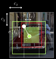 _Passthrough Layer in YOLO V2_: Here we use fine grained features for better localization on smaller objects for this we add - `13 x 13` Prediction Layer(Say C1) for prior boxes for large scale - And another `26 x 26` Prediction Layer(Say C2) for prior boxes of smaller scale - Here we use rearrange to move from `26 x 26` of C2 to `13 x 13` of C1, now as they're of same size we concatenate them to `(4C2 + C1) x 13 x 13` and this concatenate layer has lower as well as higher rest features to make better predictions for small scale objects 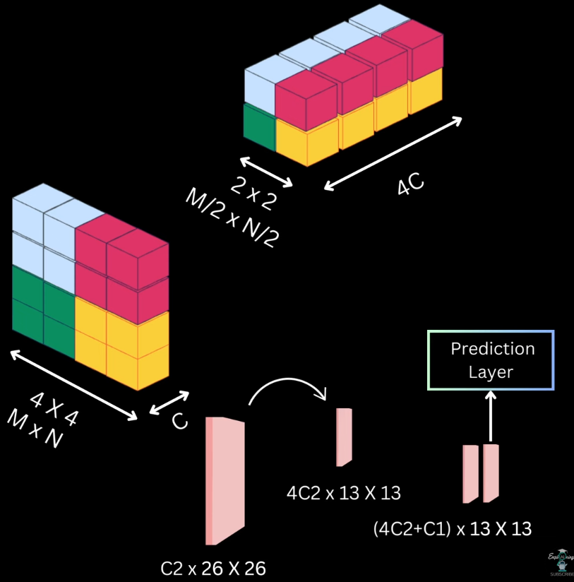 _Multi Scale Training_: In YOLO V1 we resize the images to 448 x 448 at last, but in YOLO V2 we intake images of different resolutions, like a resolution in a batch and train them, and these different sizes of images gives different results - lower resolution images gives less accurate detection but are fast - high resolution images gives high accurate detection but are slow _YOLO V2 Architecture_: Wrt YOLO V1, it's just switching from Darknet-19 as the base network 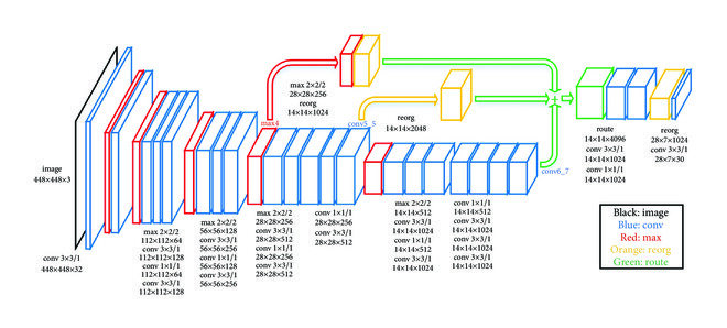 _YOLO 9000_: Most of the detection datasets, cater to a small number of object categories, The main reason for this is that detection annotation is costly but the classification annotation on the other hand is relatively cheaper (that's why we have few images but wide variety of classes) To Solve this. Authors of YOLO V2 used joint training and detection using YOLO V2 we're able to detect more than 9000 categories, the idea here is to use large available classification of data to strengthen our object detector #Q How to train on both simultaneously when only 44 ImageNet classes appear in COCO? #A Inspired by WordNet structure, YOLO9000 builds a hierarchical tree of concepts ```text Entity | |———————————————|———————————————| Dog Cat Vehicle | | | Terrier Siamese Car | | | Norfolk Airedale Bengal Persian Ferrari ``` Key insight: Convert flat 1000 ImageNet classes into a WordTree with 1369 nodes (1000 leaf nodes + 369 parent nodes) Softmax at Hierarchical Levels: Instead of one global softmax, predict conditional probabilities at each node. At the "terrier" node, predict: - Pr(Norfolk terrier | terrier) - Pr(Airedale terrier | terrier) - Pr(Lakeland terrier | terrier) To get absolute probability: `Pr(Norfolk terrier) = Pr(terrier ∣ dog) × Pr(dog ∣ entity)` Joint Training Strategy: Using only 3 anchor boxes (instead of 5) to limit output size. For detection images (COCO): - Backpropagate full YOLOv2 loss: bounding box loss + objectness loss + classification loss For classification images (ImageNet): - Backpropagate only classification loss at or above the corresponding hierarchy level - Bounding box predictions are not updated This clever scheme allows the model to learn detection features from limited labeled data and generalize to 9000+ unseen classes using classification data _Loss Function_: YOLO9000 uses a composite loss function:

L = \lambda_{coord} , L_{bbox}

• \lambda_{obj} , L_{objectness}

• \lambda_{class} , L_{classification}

Bounding Box Loss (Coordinates):

L_{bbox} = \sum_{i=0}^{S^2} \sum_{j=0}^{B} \mathbb{1}_{ij}^{obj} \Big[ (x_i - \hat{x}_i)^2 - (y_i - \hat{y}_i)^2 - (\sqrt{w_i} - \sqrt{\hat{w}_i})^2 - (\sqrt{h_i} - \sqrt{\hat{h}_i})^2 \Big] $$ Note: The square root of width and height is used to penalize large and small bounding boxes equally Objectness Loss:

L_{obj} =
\sum_{i=0}^{S^2}
\sum_{j=0}^{B}
(C_i - \hat{C}_i)

$$ClassificationLoss:(Onlyforcellsthatcontainobjects)$$

L_{class} =
\sum_{i=0}^{S^2}
\mathbb{1}i^{obj}
\sum{c \in classes}
\big(p_i(c) - \hat{p}_i(c)\big)

$$IndicatorFunction:$$

\mathbb{1}_{ij}^{obj} =
\begin{cases}
1 & \text{if an object exists in cell } i \text{ for box } j \
0 & \text{otherwise}
\end{cases}

#### Approach 8: _YOLO V3_ This is just a small set of incremental improvements over YOLO V2 - With the most important change being to move from darknet-19 to darknet-53 - And rather than doing predictions at final feature map, we do predictions at three different stages. Here - We have more number of layers - And we have residual connections in the network - And instead of Max pooling we have strided convolutions to allow network to learn in a manner that is best suited for the task  - In YOLO V3 we ignore anchors if they overlap(>threshold) with ground truth but are not the best anchor for that ground truth - The Objectness target during training is either 0 or 1 - For classification, authored have model the problem as multi-label classification where rather than softmax they predict classification scores for each class independently using sigmoid and trained using BCE loss #### Approach 9: _YOLO V4_ By the time of YOLO V4 most object detectors used in architecture that could be divided into three parts: 1. _Backbone_ which is often pre-trained on a large classification data set to act as a strong feature extractor for the detection task 2. _Neck_ which is tasked with refining features extracted from backbone and commonly also Aggregates the features extracted at various stages of backbone the main purpose of this aggregation is to enhance semantic and localization information across all scales 3. _Head_ is the last part that takes in the features from neck and finally predicts the bounding boxes and class information The Authors of YOLO V4 also experimented with bunch of features and techniques to reach to the combination of features that ends up with the best detector, which they've grouped into 1. _Bag of Freebies_: Methods that do not increase inference cost but may increase training cost and end up producing a more accurate detector. for example, data augmentation, better loss,.. 2. _Bag of Specials_: Methods that increase the inference cost by a small margin but improve accuracy of detector significantly. for example, adding attention, feature aggregation in neck which YOLO V3 does using fpn,.... Here are the strategies that derived from the above groups, which are used during image pre-training stage to boost the classification accuracy and end up with the stronger feature extractor - Bag of Freebies Strategies 1. _CutMix_: It's a `data augmentation` method - During classification training, our data points will have ground truth class label as "one" and rest all class labels will be "zero" - But in Cutmix, we mix patches of two images, by overlaying a patch of the image onto another - For, Implementing cut mix, we decide what would be our overlay regions width and height and the starting point of our overlaid region then for pixels belonging to that region we simply overlay the pixels of a different image onto this one the ground truth label in Cut mix is now mixed proportionally according to the area of patches - Because this model is trained on a mixture of images the classifier is forced to attend on non-discriminative parts of objects like legs of dog rather than face and hence ends up being more generalizable furthermore it gives the model the ability to identify objects from their partial views which will definitely benefit in cases where the object itself is occluded - This augmentation strategy ends up with a better classifier where we get close to 2% Improvement on classification accuracy and when this classified network is used as a pre-trained model for detection fine-tuning stage we end up with performance gains in detection as well -  2. _Mosaic_: Again a `data augmentation` strategy which is very similar to cut mix - It combines four different images into a single training image - For classification: - A random point splits the input image into four regions - Each region is filled with a patch from a different image - The final label is a weighted sum of the original labels, proportional to each patch’s area - For detection: - Four images are placed on a canvas twice the input width and height - A random center point determines placement, and the final image is cropped to the required size - Bounding boxes are adjusted accordingly - This helps to Improve robustness to occlusion and Helps the model learn objects in varied contexts, for both classification and detection tasks -  3. _DropBlock_: It's a regularization technique designed specifically for convolutional neural networks, addressing limitations of standard Dropout on image feature maps - In CNNs, spatially adjacent activations are highly correlated - Standard Dropout removes random individual activations, but semantic information can still be inferred from neighbors - Spatial Dropout improves this by dropping entire feature maps, but it is often too aggressive - DropBlock removes contiguous regions of a feature map, forcing the network to learn robust, distributed representations - Instead of dropping isolated activations, DropBlock zeros out continuous square regions of size `block_size × block_size`, effectively removing meaningful semantic parts (e.g., an object’s head) - `Algorithm`: 1. Initial Mask Sampling - Sample a smaller binary mask using Bernoulli distribution with probability `γ` - Mask contains 1s for regions to drop, 0s otherwise 2. Why Smaller Mask? - Ensures each sampled 1 can expand fully inside the feature map - Prevents edge bias during block expansion 3. Zero Padding - Pad the mask to match feature map dimensions 4. Block Expansion - Apply Max Pooling with: - Kernel size = `block_size` - Padding = `block_size // 2` - This expands each sampled 1 into a full block 5. Mask Inversion - Flip the mask so: `0 → dropped`, `1 → kept` 6. Apply to Feature Map - Multiply the flipped mask with the feature map - Scale remaining activations (as in standard Dropout) 7. Channel-wise Masks - Each channel uses an independent mask - Shared masks across channels perform worse

\gamma = \frac{1 - \text{keep_prob}}{\text{block_size}^2} \cdot \frac{\text{feat_size}^2}{(\text{feat_size} - \text{block_size} + 1)^2}

$$4{.}_{S}moothLabelin{g}_{:}Thisisachangeingroundtruthlabelsusedforclassificationtrainingi{t}^{\prime }sacommonideathatismeanttotackleoverfittingofnetworkandactasa‘Regularizer‘-Standardclassificationusesone-hotlabels-Cross-entropylosspushesthemodeltomatchthisharddistribution-Toapproachone-hottargets,themodelincreaseslogitsforthecorrectclass,leadingtooverconfidentpredictionsandlargeweights-Labelsmoothingsoftensthetargetdistribution,actingasaregularizer-TheCoreIdea:Insteadofassigningprobability‘1‘tothecorrectclassand‘0‘toothers:-Reducethecorrectclassprobabilityslightly-Distributetheremainingprobabilitymassuniformlyacrossotherclasses-Thisdiscouragesextremelogitvaluesandimprovesgeneralization-‘q_i‘\to target(label)distribution-‘p_i‘\to predictedprobabilityforclass‘i‘$$

L = -\sum_i q_i \log p_i

$$-SoftmaxProbability:-‘z_i‘\to logitforclass‘i‘$$

p_i = \frac{e^{z_i}}{\sum_j e^{z_j}}

$$-LabelSmoothingFormula-‘LS‘\to labelsmoothingfactor-‘K‘\to numberofclasses$$

y_{\text{smooth}} = y_{\text{true}} (1 - \text{LS}) + \frac{\text{LS}}{K}

$$-BagofSpecialsforBackbone1{.}_{M}ishActivatio{n}_{:}Mishisasmooth,non-monotonicactivationfunctionproposedasaself-regularizingalternativetoReLUandSwish,particularlyeffectiveindeepvisionmodels$$

\text{Mish}(x) = x \cdot \tanh(\text{softplus}(x))

\text{softplus}(x) = \ln(1 + e^x)

$$-Forlargepositive‘x‘:-‘softplus(x)\approx x‘-‘tanh(x)\approx 1‘-\Rightarrow ‘Mish(x)\approx x‘-Forlargenegative‘x‘:-‘softplus(x)\approx 0‘-‘tanh(0)\approx 0‘-\Rightarrow ‘Mish(x)\approx 0‘2{.}_{C}ross-StagePartialConnection{s}_{:}CSPconnectionssplitfeaturemapsacrossstagestoreducecomputation,improvegradientflow,andavoidduplicategradientinformation-IntroducedusingDenseNetasbackbone,laterextendedtoResNet-styleblocks,andadoptedinYOLOv4(CSPDarknet53)-CoreIdea:-Splitinputfeaturemapalongthechanneldimension-Onepartgoesthroughablock(e.g.,residualblock)-Otherpartbypassescomputation-Concatenatebothpartsandapplyatransitionlayer-CSPResidualBlockMath:1.Theinputfeaturemapbe:$$

X \in \mathbb{R}^{H \times W \times C}

$$2.ChannelSplit$$

X_1, X_2 = \text{Split}(X), \quad C_1 = C_2 = \frac{C}{2}

$$3.ResidualProcessing$$

Y = \text{ResBlock}(X_1)

$$4.TransitionLayer(BeforeConcatenation)$$

Y’ = \text{Conv}_{1\times1}(Y)

$$5.Concatenation$$

Z = \text{Concat}(Y’, X_2)

$$6.FinalTransitionLayer$$

\text{Output} = \text{Conv}_{1\times1}(Z)

$$-CSPDarknet53(YOLOv4Backbone)-CSPDarknet53=Darknet53+CSPblocks-OriginalDarknetblock:Downsample\to Residualblocks\to Downsample-CSPversion:-Downsample\to Split-Onepart\to Residualblocks\to 1\times 1Conv-Otherpart\to Bypass-Concatenate\to 1\times 1Conv\to Downsample-3{.}_{M}ultiInputWeightedResidualConnection{s}_{:}Thistechniqueisdesignedforcross-scalefeaturefusion,i.e.,combiningfeaturemapsofdifferentspatialresolutions,asusedintheEfficientDetneck(BiFPN)-CoreIdea-Eachinputfeatureisassignedalearnableweight-Thenetworklearnsfeatureimportanceduringtraining-Supports:-Per-featureweights(onescalarperinput)-Per-channelweights(oneweightperchannel)-GeneralFusionFormula:For‘N‘inputfeatures:$$

Y = \sum_{i=1}^{N} w_i \cdot X_i

$$-‘X_i‘\to inputfeaturemaps(alignedinresolution)-‘w_i‘\to learnableweights-FusionVariants1.UnboundedFusion$$

Y = \sum_{i=1}^{N} w_i X_i

$$-Nonormalization-Weightscanbenegativeorlarge-Lessstableduringtraining2.SoftmaxFusion$$

\alpha_i = \frac{e^{w_i}}{\sum_{j=1}^{N} e^{w_j}}

Y = \sum_{i=1}^{N} \alpha_i X_i

$$-Weightsnormalizedto‘[0,1]‘-Sumofweights=1-Stablebutcomputationallyheavier3.FastNormalizedFusion(EfficientDet/YOLOv4)$$

\hat{w}_i = \text{ReLU}(w_i)

Y = \frac{\sum_{i=1}^{N} \hat{w}i X_i}{\sum{i=1}^{N} \hat{w}_i + \epsilon}

$$-Ensuresnon-negativeweights-Avoidssoftmax-Fasterandstable-Mostcommonlyusedinpractice-BagofFreebiesforDetector1{.}_{C}rossMini-B{N}_{:}BatchNormalization(BN)normalizesactivationsusingbatchstatisticstoimproveconvergence$$

\mu_B = \frac{1}{m}\sum_{i=1}^{m} x_i

\sigma_B^2 = \frac{1}{m}\sum_{i=1}^{m}(x_i - \mu_B)

\hat{x}_i = \frac{x_i - \mu_B}{\sqrt{\sigma_B^2 + \epsilon}}

y_i = \gamma \hat{x}_i + \beta

$$-Workswellforlargebatchsizes-Becomesnoisyforsmallbatches(commoninobjectdetection)-FromBN\to CBN\to CmBN1.BatchNormalization-Statisticscomputedperbatch-Weightsupdatedaftereachbatch2.Cross-IterationBatchNorm(CBN)-AggregatesstatisticsfrompastKbatches-Requiresweight-changecompensation-Complexandcostly3.CrossMini-BatchNorm(CmBN)–YOLOv4-Aggregatesstatisticswithinasinglebatch-Noweightcompensationneeded-Weightsupdatedonceperfullbatch-CmBNAlgorithm(PerMini-Batch)1.Computemeanandvarianceforcurrentmini-batch2.Aggregatestatisticsfrompreviousmini-batches3.Normalizeactivationsusingaggregatedstatistics4.Accumulategradients(noweightupdateyet)5.Updateweightsafterlastmini-batch-AggregationCoefficient$$

\alpha_t = \frac{1}{t+1}

$$-‘t‘=mini-batchindex(startingfrom0)-AggregatedMeanFormula$$

\mu_t^{agg} = \alpha_t \mu_t + (1 - \alpha_t)\mu_{t-1}^{agg}

$$-Firstmini-batch:$$

\mu_0^{agg} = \mu_0

$$-AggregatedVariance(Conceptual)$$

\sigma_t^{2,agg} = \alpha_t \sigma_t^2 + (1 - \alpha_t)\sigma_{t-1}^{2,agg}

$$-NormalizationUsingAggregatedStatistics$$

\hat{x} = \frac{x - \mu_t^{agg}}{\sqrt{\sigma_t^{2,agg} + \epsilon}}

$$2{.}_{C}ompleteIOULos{s}_{:}-WhyMSEIsNotIdealforBoxRegression:UsingMSEonboxcoordinates(‘x1,y1,x2,y2‘or‘x,y,w,h‘)hasmajorissues:-SameMSEcancorrespondtoverydifferentoverlaps-Notscale-invariant-Optimizescoordinatedistance,notoverlapquality-Doesnotreflectlocalizationqualitydirectly-‘IoULoss‘:Todirectlyoptimizeoverlap:$$

\text{IoU} = \frac{|B \cap B^{gt}|}{|B \cup B^{gt}|}

\mathcal{L}_{IoU} = 1 - \text{IoU}

$$-Limitation-Allnon-overlappingboxesgetidenticalloss-Nonotionof"howfar"boxesare-‘GeneralizedIoU(GIoU)‘-Addsapenaltyfornon-overlappingcases.$$

\text{GIoU} = \text{IoU} - \frac{|C - (B \cup B^{gt})|}{|C|}

\mathcal{L}_{GIoU} = 1 - \text{GIoU}

$$-Where:$$

C = \text{smallest enclosing box of } B \text{ and } B^{gt}

$$-Limitation-Whenoneboxenclosestheother,GIoUreducestoIoU-Doesnotconsidercenterdistanceoraspectratio-‘DistanceIoU(DIoU)‘-Addressescentermisalignment$$

\text{DIoU} = \text{IoU} - \frac{\rho^2(b, b^{gt})}{c^2}

\mathcal{L}_{DIoU} = 1 - \text{DIoU}

$$-Where:$$

\rho(b, b^{gt}) = \text{Euclidean distance between box centers}

c = \text{diagonal length of enclosing box } C

$$-Benefits-Fasterconvergence-Handlesbothoverlappingandnon-overlappingcases-Stillignoresaspectratio-‘CompleteIoU(CIoU)‘-Addsaspectratioconsistency$$

\text{CIoU} = \text{IoU}

• \frac{\rho^2(b, b^{gt})}{c^2}
• \alpha v

\mathcal{L}_{CIoU} = 1 - \text{CIoU}

$$-‘AspectRatioPenalty‘$$

v = \frac{4}{\pi^2} \left( \arctan\frac{w^{gt}}{h^{gt}} - \arctan\frac{w}{h} \right)

\alpha = \frac{v}{(1 - \text{IoU}) + v}

$$|Loss|Overlap|Distance|AspectRatio|Convergence||----|-------|----------|------------|-----------||MSE|❌|❌|❌|Slow||IoU|✅|❌|❌|Medium||GIoU|✅|✅(coarse)|❌|Better||DIoU|✅|✅|❌|Faster||CIoU|✅|✅|✅|Fastest|3{.}_{S}elfAdversarialTrainin{g}_{:}Self-AdversarialTrainingimprovesmodelrobustnessbyintentionallyconfusingthenetworkwithitsowngradients,thentrainingittorecoverfromthatconfusion.UsedinYOLOv4asaregularizationandrobustnesstechnique.-CoreIdea:Traininghappensintwostagesperimage:1.Attackstage–modifytheimagetofoolthemodel2.Defensestage–trainthemodeltocorrectlypredictonthemodifiedimage-Themodeleffectivelyattacksitself,thenlearnstoresistthatattack-Stage1:AdversarialImageGeneration-Freezenetworkweights-Useincorrectlabels(e.g.,“noobject”)-Computelossandgradientsw.r.t.theinputimage-Perturbtheimagetoreducecorrectdetection-Loss(WrongLabel)$$

\mathcal{L}{adv} = \mathcal{L}(f\theta(x), y_{\text{fake}})

$$-ImagePerturbation$$

x’ = x + \epsilon \cdot \text{sign} \left( \nabla_x \mathcal{L}_{adv} \right)

$$-‘x‘\to originalimage-‘x^{\prime }‘\to adversarialimage-‘\epsilon ‘\to perturbationstrength-Weights‘\theta ‘remainunchanged-Stage2:RobustTraining-Feedadversarialimage‘x^{\prime }‘-Usecorrectground-truthlabels-Updatenetworkweightstorecovercorrectpredictions-Loss(TrueLabel)$$

\mathcal{L}{sat} = \mathcal{L}(f\theta(x’), y_{\text{true}})

\theta \leftarrow \theta - \eta \nabla_\theta \mathcal{L}_{sat}

$$4{.}_{G}ridSensitivit{y}_{:}-YOLOv3CenterPrediction:InYOLOv3,theboundingboxcenterispredictedas:$$

x = C_x + \sigma(t_x), y = C_y + \sigma(t_y)

- `C_x, C_y` → top-left coordinates of the grid cell - `t_x, t_y` → raw network outputs - `σ(.)` → sigmoid function - Output range of `σ(.)` is (0, 1) - This ensures the box center lies inside the grid cell #Q Why Grid Sensitivity Occurs ? #A Boundary Case Problem - If the ground-truth box center lies on a grid boundary, e.g.: - exactly at `C_x` - or exactly at `C_x + 1` - Then the model needs: $$ \sigma(t_x) = 0 \quad \text{or} \quad \sigma(t_x) = 1 $$ - Sigmoid Limitation: Sigmoid never outputs exact 0 or 1 - `σ(-4) ≈ 0.018` - `σ(-10) ≈ 0.000045` - `σ(+4) ≈ 0.982` - `σ(+10) ≈ 0.99995` - To approach 0 or 1, the network must predict very large |tₓ| values. - This causes: - Hard optimization near grid boundaries - Unstable gradients - Poor localization for boundary objects - This issue is called grid sensitivity - YOLOv4 Solution: Scaled Offset Prediction - YOLOv4 modifies the center prediction formula: $$ x = C_x + \alpha \cdot \sigma(t_x) - \frac{\alpha - 1}{2}, y = C_y + \alpha \cdot \sigma(t_y) - \frac{\alpha - 1}{2} $$ Where: `α > 1` (scaling factor) - Summary: - Problem: Sigmoid-bounded offsets in YOLOv3 make boundary box prediction difficult - Cause: Sigmoid cannot output exact 0 or 1 - Solution (YOLOv4): Scale sigmoid output with `α > 1` - Benefit: - Reduced grid sensitivity - Easier optimization - Better localization near grid boundaries 5. _Genetic Algorithm_: YOLOv4 uses a genetic algorithm (GA) to automatically find optimal hyperparameters, instead of relying on manual tuning. Examples of tuned hyperparameters: Learning rate, Momentum, Weight decay, Data augmentation probabilities (mosaic, hue, saturation, flip, etc.), Loss-related scaling factors 1. Initialization - Start with an initial population of hyperparameter sets - These can be: - Default values - Slight random variations around known good values 2. Training & Fitness Evaluation - For each hyperparameter set: 1. Train the YOLO model using those hyperparameters 2. Evaluate performance on validation data 3. Compute a fitness score 3. Fitness Score Definition - Fitness reflects how good a hyperparameter set is - It is computed as a weighted sum of multiple metrics, such as:

\text{Fitness} = w_1 \cdot \text{Precision} + w_2 \cdot \text{Recall} + w_3 \cdot \text{mAP}

$$-‘w_1,w_2,w_3‘arepredefinedweights-Metricslikeprecision,recall,mAPareallconsidered-Thisallowsbalancingdetectionquality,notjustonemetric4.Selection(SurvivaloftheFittest)-Oncefitnessscoresarecomputed:-SelecthyperparametersetsfromthetopNperformers-Selectionstrategies:-RandomselectionfromtopN-Weightedselectionwherehigherfitness\Rightarrow higherprobability-Thisselectedsetbecomestheparentforthenextgeneration5.Mutation:-Theselectedhyperparametersetismutated:-Eachhyperparameterhas:-Mutationprobability\to howoftenitchanges-Mutationvariance\to howmuchitchanges-Example:-Learningratemaychangeby\pm 10-Augmentationprobabilitymayshiftslightly-Mathematically:‘ne{w}_{v}alue=ol{d}_{v}alue+Normal(0,variance)‘6.EvolutionAcrossGenerations:ThisprocessisrepeatedforKgenerations:-Typically:K\approx 100–300-Overtime:-Poormutationsdieout-Beneficialmutationssurvive-Fitnesssteadilyimproves7.FinalResult-Afterallgenerations:-Thebest-performinghyperparametersetisselected-ThisbecomesthefinalconfigurationfortrainingYOLOv4-BagofSpecialsforDetector1{.}_{S}patialPyramidPoolin{g}_{:}-Givenabackbonefeaturemap(F):1.Applymaxpoolingwithmultiplelargekernelsizes:‘5x5‘,‘9x9‘,‘13x13‘-Use:Stride=1,Padding=kerne{l}_{s}ize/2(topreservespatialdimensions)-FeatureConcatenation:Allpooledfeaturesareconcatenatedalongthechanneldimension:$$

F_{\text{SPP}} = \text{Concat}\left( F,; \text{MaxPool}{5\times5}(F),; \text{MaxPool}{9\times9}(F),; \text{MaxPool}_{13\times13}(F) \right)

- Spatial size remains the same - Channel depth increases - Each pooled feature captures context at a different scale - Intuition - Small kernels → local details - Large kernels → global context - Concatenation allows the network to choose what context matters 2. _Spatial Attention Module_: - SAM is inspired by CBAM (Convolutional Block Attention Module) - CBAM uses two attention mechanisms: Channel Attention, Spatial Attention - YOLOv4 uses a simplified version focusing on spatial (point-wise) attention only - `Channel Attention` (What to focus on) #Q Which feature channels are most important? #A Process: 1. Input feature map $$ F \in \mathbb{R}^{C \times H \times W} ) $$ 2. Apply: - Global Average Pooling → ( C x1 x 1 ) - Global Max Pooling → ( C x 1 x 1 ) 3. Pass both through a shared MLP 4. Add outputs and apply sigmoid 5. Multiply with input feature map

M_c(F) = \sigma(\text{MLP}(\text{AvgPool}(F)) + \text{MLP}(\text{MaxPool}(F)))

- Output: C x H x W - `Spatial Attention` (Where to focus) #Q Where is the informative region in the feature map? #A Process: 1. Apply: - Channel-wise Average Pooling → ( 1 x H x W ) - Channel-wise Max Pooling → ( 1 x H x W ) 2. Concatenate → ( 2 x H x W ) 3. Apply 7×7 convolution 4. Apply sigmoid 5. Multiply with input feature map

M_s(F) = \sigma(\text{Conv}_{7\times7}([\text{AvgPool}_c(F), \text{MaxPool}_c(F)]))

- Output: ( C x H x W ) - `SAM in YOLOv4` (Simplified Attention) - YOLOv4 does NOT use full CBAM - Instead, it introduces a lightweight Spatial Attention Module (SAM) - SAM Operation: - Given input feature map $$ F \in \mathbb{R}^{C \times H \times W} $$ 1. Apply 1×1 convolution with: Number of filters = ( C ) 2. Apply sigmoid activation 3. Multiply element-wise with original input

M_{\text{SAM}}(F) = \sigma(\text{Conv}_{1\times1}(F))

F’ = F \odot M_{\text{SAM}}(F)

$$3{.}_{P}athAggregationNetwor{k}_{:}-YOLOv3Neck=FPN-Usestop-downpathway-Combines:-Low-resolution,semanticallystrongfeatures-High-resolution,semanticallyweakfeatures-Helpssmallobjectdetection-LimitationofFPN:-Informationflowfromlow-level\to high-levelfeaturesisweak-Pathfromearlylayerstodeeplayersislong-Low-levelfeatures(richinlocalization)areunderutilizedforlargeobjects-CoreIdea:Improveinformationpropagationbyaddingabottom-uppathinadditiontoFPN’stop-downpath-SoPANethas:-Top-DownPath(sameasFPN)-Bottom-UpPath(new,shorterpath)-Thisenables:-Betterlocalization-Strongerfeaturefusion-Improveddetectionaccuracy-PANetArchitecture(Concept)1.Top-DownPath(FPN)-SameasYOLOv3:High-levelsemanticfeaturesarepasseddowntohigher-resolutionlayers2.Bottom-UpPath(New)-Goal:Provideashorterpathforlow-levelfeaturestoreachhigherlevels-Process(YOLOv4-style):1.Takehigher-resolutionfeaturefromalowerlayer2.Downsampleit(stride-2convolution)3.Concatenatewithsame-resolutionfeaturefromtop-downpath4.Applyconvolutionblocks5.Usethesefeaturesforfinalpredictions-FeatureFlow:Backbone\to Top-DownPath(FPN)\to Bottom-UpPath(PAN)\to DetectionHeads-4{.}_{d}IOUNM{S}_{:}TraditionalNMSsuppressesboxessolelybasedonIoUoverlap,thiscausesfalsesuppression,especiallywhen:-Objectsarecloseoroccluded-Twodistinctobjectshavehighoverlap-Overlapaloneisnotsufficienttojudgeduplication-CoreIdea:InsteadofusingonlyIoU,DIoU-NMSalsoconsidersthedistancebetweenboxcenters-Boxeswithfar-apartcentersarelikelydifferentobjects-EvenifIoUishigh,suchboxesshouldnotbesuppressed-DistancePenaltyTerm(fromDIoULoss)-b=candidatebox-M=highestscoringbox-p(c)=Euclideandistancebetweenboxcenters-c=diagonallengthofthesmallestenclosingbox$$

\text{DistancePenalty}(b, M) = \frac{\rho^2(\text{center}_b, \text{center}_M)}{c^2}

$$-DIoUMetricUsedinNMS$$

\text{DIoU}(b, M) = \text{IoU}(b, M) \frac{\rho^2(\text{center}_b, \text{center}_M)}{c^2}

$$-DIoU-NMSSuppressionRule:Abox(b)issuppressedonlyif:$$

\text{DIoU}(b, M) > \tau

- This means: - High overlap alone is not enough - Large center distance reduces suppression score - Here we take a key assumption that, boxes with large center distance likely correspond to different objects, even if they overlap. - 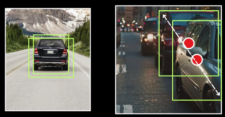 ##### YOLO V4 Architecture 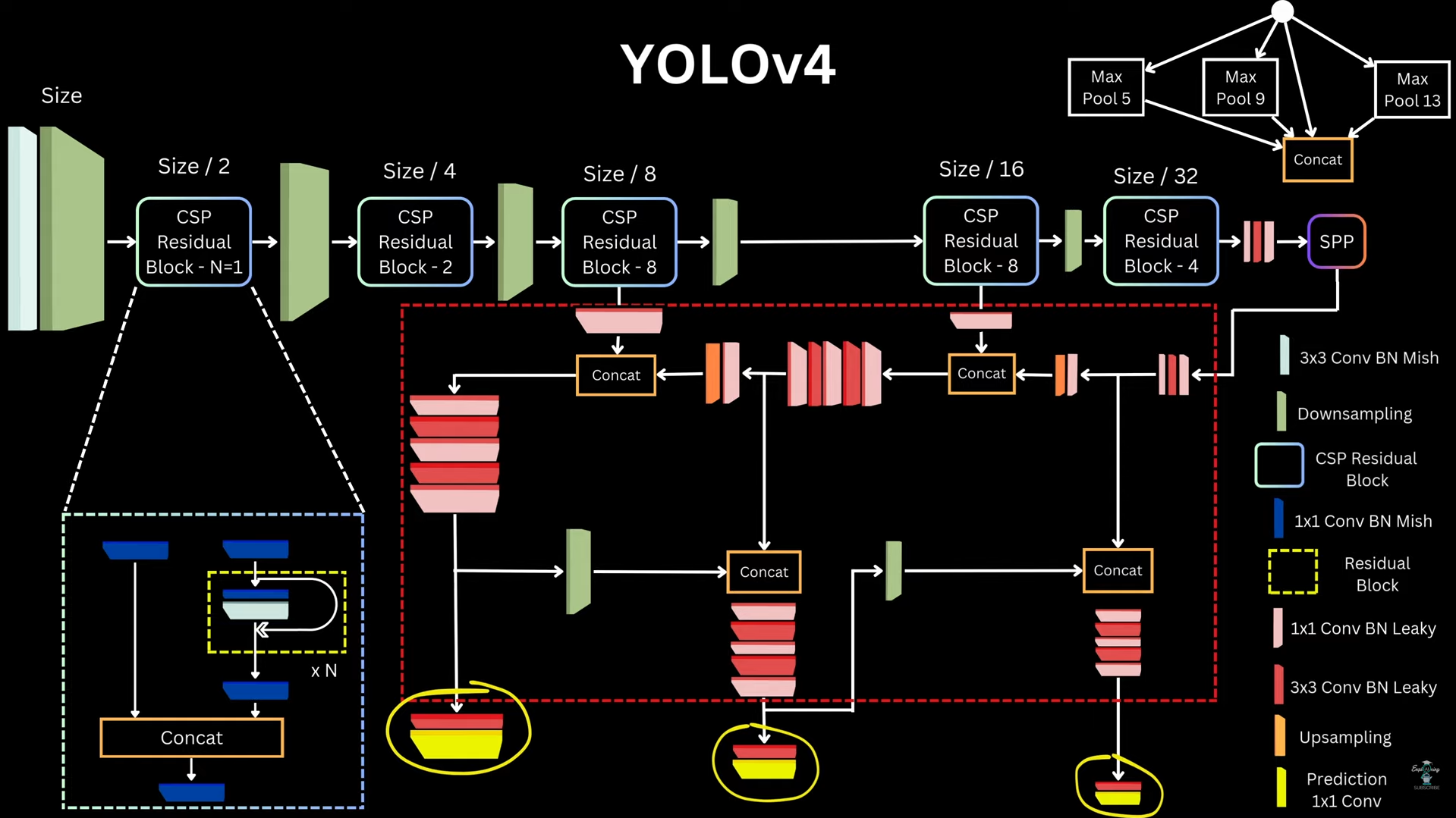 #### Approach 10: _YOLO V5_ ##### YOLO V5 Architecture 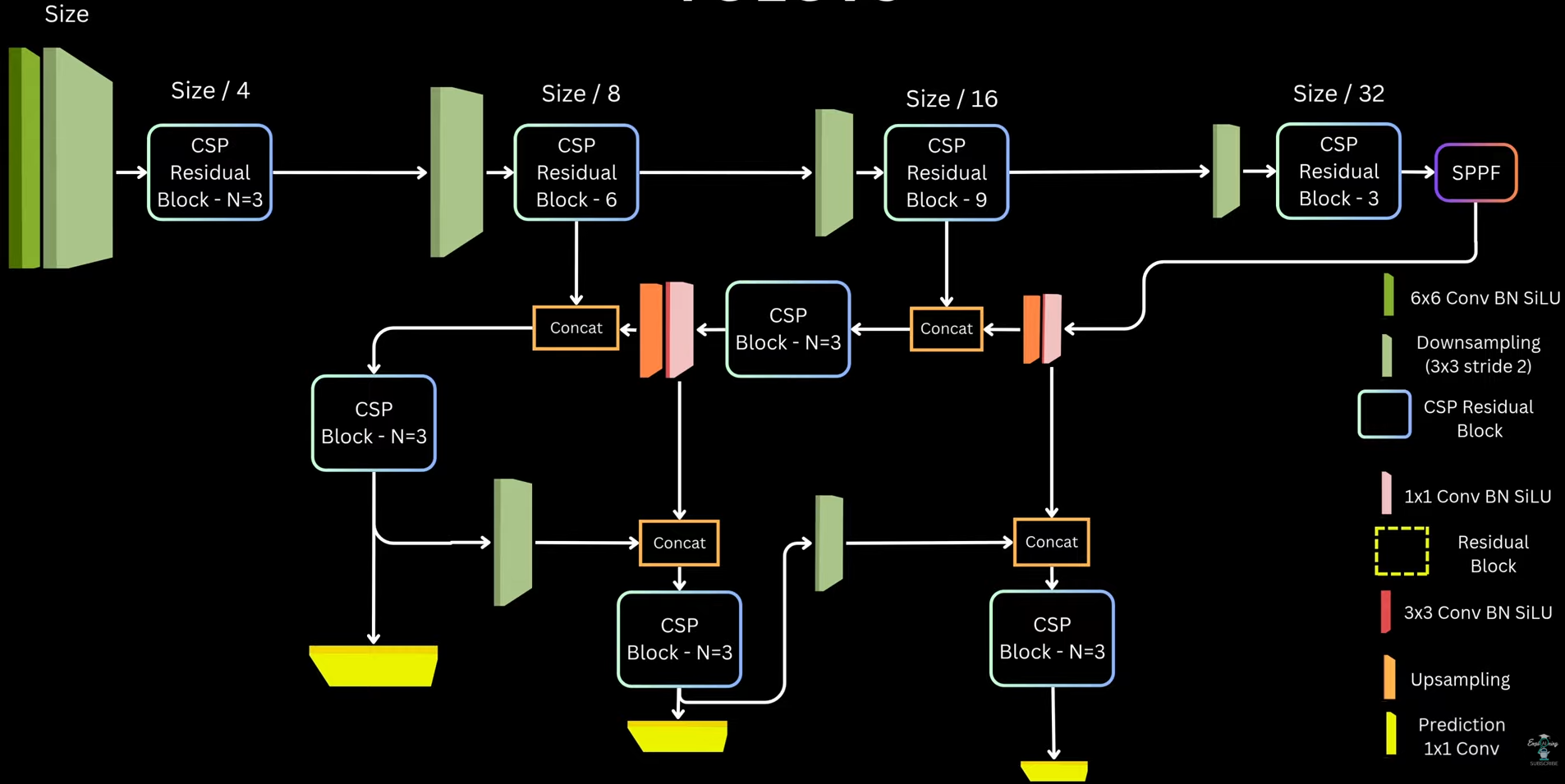 ##### Matching Targets and Prediction _Predictions_: Like YOLOv3/v4, for each grid cell and each anchor, YOLOv5 predicts: `(5 + C) values` - 4 box parameters → bounding box transformation - 1 objectness score → probability that an object exists - C class probabilities _Bounding Box Parameterization_: 1. Center coordinates (x, y) - YOLOv5 uses the same modified formulation as YOLOv4 to reduce grid sensitivity

\begin{aligned}
b_x &= (2 \cdot \sigma(t_x) - 0.5) + c_x \ b_y &= (2 \cdot \sigma(t_y) - 0.5) + c_y
\end{aligned}

- σ: sigmoid, c_x, c_y: top-left coordinates of the grid cell, Range of offsets: (-0.5, 1.5) - This allows prediction of box centers near or across grid boundaries, without requiring sigmoid outputs to be exactly 0 or 1 2. Width and Height (Major change in YOLOv5) - Unlike YOLOv3/v4 (where width & height were unbounded), YOLOv5 bounds them using sigmoid

\begin{aligned}
b_w &= a_w \cdot (2 \cdot \sigma(t_w))^2 \ b_h &= a_h \cdot (2 \cdot \sigma(t_h))^2
\end{aligned}

$$-a_w,a_h:anchorwidthandheight-Since\sigma (t)\in (0,1):b_w,b_h\in (0,4xanchorsize)-Thisstabilizestrainingandpreventsextremeboxsizes3.YOLOv5AnchorMatching(Ratio-based)-YOLOv5doesnotuseIoUforanchormatching-Width–HeightRatioCheck-Foraground-truthboxandanchorbox:$$

\max\left(
\frac{w_{gt}}{w_a}, \frac{w_a}{w_{gt}},
\frac{h_{gt}}{h_a}, \frac{h_a}{h_{gt}}
\right) < t

- (t) = anchor threshold (default 4) - An anchor is matched if its dimensions are within (1/4, 4) of the GT box Implications of Ratio-based Matching 1. IoU is irrelevant for matching → Anchor can be matched even if it doesn’t overlap the GT box 2. Multiple anchors can match the same ground truth 3. One anchor can be matched to multiple ground truths 4. Small objects naturally match small anchors on high-resolution feature maps This improves recall, especially for small objects ##### Grid Cell Assignment in YOLOv5 - Traditional YOLO: Only the grid cell containing the GT center is responsible - YOLOv5: Multiple Responsible Grid Cells: Because center offsets can now lie in (-0.5, 1.5), adjacent grid cells can also predict the same GT box - How it works: 1. Find the main grid cell containing the GT center 2. Divide that cell into four quadrants 3. Depending on where the GT center lies: Include up to 2 adjacent grid cells 4. Grid cells are included only if they exist (not at borders) - This results in: - 1 to 3 grid cells responsible for the same GT box - Each with multiple valid anchors - Improves learning near grid boundaries and stabilizes training _Summary_: For each ground truth box: 1. Select anchors that satisfy width–height ratio constraint 2. Find center grid cell 3. Add adjacent grid cells based on center location 4. For each (grid cell, anchor) pair: - Assign the same ground truth box - Train box regression, objectness, and class prediction ##### YOLO V5 Loss YOLOv5 uses a multi-part loss computed over predictions from multiple detection layers. The total loss is a combination of: 1. _Localization (Bounding Box) Loss_: - YOLOv5 uses Complete IoU (CIoU) loss for localization - Predicted box formulation: - For a grid cell at location (c_x, c_y) and anchor (a_w, a_h): - Center coordinates

\begin{aligned}
b_x &= (2 \cdot \sigma(t_x) - 0.5) + c_x \ b_y &= (2 \cdot \sigma(t_y) - 0.5) + c_y
\end{aligned}

$$-Widthandheight$$

\begin{aligned}
b_w &= a_w \cdot (2 \cdot \sigma(t_w))^2 \
b_h &= a_h \cdot (2 \cdot \sigma(t_h))^2
\end{aligned}

$$-CIoULoss$$

\mathcal{L}{\text{box}} = 1 - \text{CIoU}(B{pred}, B_{gt})

$$-CIoUincorporates:IoUoverlap,Centerdistance,Aspectratioconsistency-Localizationlossiscomputedonlyforforeground(matched)boxes1.ObjectnessLoss2.ClassificationLoss-Eachiscomputedperdetectionlayerandthenaggregated2{.}_{O}bjectnessLos{s}_{:}-Objectnesspredictswhetheranobjectexistsinagivenanchor-gridcellpair-Targetvalues-Foregroundboxes:$$

y_{obj} = \text{IoU}(B_{pred}, B_{gt})

$$-Backgroundboxes:$$

y_{obj} = 0  

$$-Lossformulation:BinaryCrossEntropy(BCE)$$

\mathcal{L}{obj} = \text{BCE}(\sigma(p{obj}), y_{obj})

$$-UsingIoUastheobjectnesstargethelpsthemodellearnboxqualityawareness3{.}_{C}lassificationLos{s}_{:}-YOLOv5usesBinaryCrossEntropyforclassification(notsoftmaxCE)-Foraboxassignedtoclass(c):$$

y_c =
\begin{cases}
1 & \text{for ground truth class} \
0 & \text{for all other classes}
\end{cases}

\mathcal{L}{cls} =
\sum{c=1}^{C}
\text{BCE}(\sigma(p_c), y_c)
]

$$-Computedonlyforforegroundboxes-Supportsmulti-labelclassification(eventhoughCOCOissingle-label{)}_{F}inalYOLOv5Los{s}_{:}$$

\mathcal{L}{total} =
\lambda{box} \mathcal{L}_{box}^{total}

• \lambda_{obj} \mathcal{L}_{obj}^{total}
• \lambda_{cls} \mathcal{L}_{cls}^{total}

- lambda_{box}, lambda_{obj}, lambda_{cls} are predefined hyperparameters - The final loss is scaled by batch size (as done in the YOLOv5 repo) | Aspect | YOLOv3/v4 | YOLOv5 | | ------------------- | ------------------ | ---------------- | | Box loss | MSE / IoU variants | CIoU | | Width/height | Exponential | Bounded sigmoid² | | Objectness target | Binary (0/1) | IoU-based | | Anchor matching | IoU-based | Ratio-based | | Grid responsibility | Single cell | Multiple cells | ##### Augmentations in YOLOv5 YOLOv5 uses a rich set of augmentations defined in the COCO hyperparameter file. Most augmentations are similar to earlier YOLO versions, with a few notable additions 1. Copy-Paste Augmentation - Object segments and labels are copied from one image - They are pasted onto another image - Generates new training samples with more object diversity - Helps improve robustness, especially for rare objects 2. MixUp Augmentation - Two random images are linearly combined - Corresponding labels are also linearly combined - Encourages smoother decision boundaries - Acts as a strong regularizer 3. Mosaic Augmentation - Combines 4 or sometimes 9 images into a single image - Improves: - Multi-scale object detection - Context understanding - Particularly useful for small objects - Same idea as YOLOv4 Mosaic ##### Hyperparameter Evolution (Genetic Algorithm) YOLOv5 does automatic hyperparameter tuning using a genetic evolution algorithm _Process_: 1. Start with an initial estimate of hyperparameters 2. Train the model and compute a fitness score: Typically mAP 3. Mutate hyperparameters across generations _Key Parameters_: - Mutation probability - How often a parameter is modified - Mutation variance - How much the parameter is modified - This process is repeated for many generations to find optimal values ##### AutoAnchor in YOLOv5 Before training, YOLOv5 checks whether the provided anchors are suitable for the dataset 1. Anchor Checking - Extracts width and height of all ground-truth boxes - Randomly scales boxes to simulate data diversity 2. Anchor Fitness Metrics 1. Anchors Above Threshold - Average number of anchors per target - That satisfy width–height ratio constraints 2. Best Possible Recall (BPR) - Fraction of ground-truth boxes - For which at least one anchor satisfies the ratio constraint - If, Best Possible Recall > 0.98 → Anchors are acceptable ##### Anchor Evolution If anchors are poor: 1. Run K-Means to get initial anchors 2. Apply genetic evolution over ~1000 generations 3. Fitness score is based on anchor-to-target width - height ratio #### Note: ##### IOU (Intersection Over Union) It's used in evaluating bounding box localization accuracy in object detection, measuring the overlap between predicted and ground truth boxes

\text{IoU} = \frac{\text{Area of Intersection}}{\text{Area of Union}}

The value ranges from 0 (no overlap) to 1 (perfect match). In production, perfect IOU of 1 is extremely rare; values above 0.5 are typically considered acceptable detections ```python def get_iou(det, gt): det_x1, det_y1, det_x2, det_y2= det gt_x1, gt_y1, gt_x2, gt_y2 = gt x_left = max(det_x1, gt_x1) y_top = max(det_y1, gt_y1) x_right = min(det_x2, gt_x2) y_bottom = min(det_y2, gt_y2) if x_right < x_left or y_bottom < y_top: return 0.0 area_intersection = (x_right - x_left) * (y_botton - y_top) det area = (det_x2 - det_x1) * (det_y2 - det_y1) gt_area = (gt_x2 - gt_x1) * (gt_y2 - gt_y1) area_union = float(det_area * gt_area - area_intersection + 1E-6) iou = area_intersection / area_union return iou ``` ##### NMS (Non-Maximum Suppression) It eliminates redundant overlapping bounding boxes from object detectors, ensuring each object is detected exactly once The Algorithm is as follows: 1. Sort all predicted boxes by confidence score (descending) 2. Select the highest confidence box as a detection 3. Calculate IOU between this box and all remaining boxes 4. Suppress (discard) boxes where IOU > threshold (typically 0.5) 5. Repeat until all boxes are processed ```python def nms(dets, nms threshold=0.5): # dets [ [x1, y1, x2, y2, score], ...] # Sort detections by confidence score sorted_dets = sorted(dets, key=lambda k: -k[-1]) # List of detections that we will return keep_dets = [] while Len(sorted_dets) > 0: keep_dets.append(sorted_dets[0]) # remove highest confidence box # and remove all boxes that have high overlap with it sorted_dets = [ box for box in sorted_dets[1:] if get_iou(sorted_dets[0][:-1], box [:-1]) < nms_threshold ] return keep_dets ``` The primary hyperparameter controlling suppression aggressiveness. Lower thresholds (0.3-0.4) suppress more boxes, reducing false positives but risking missed detections in crowded scenes. Higher thresholds (0.6-0.7) allow closer boxes, useful for dense object scenarios ##### Recall and Precision 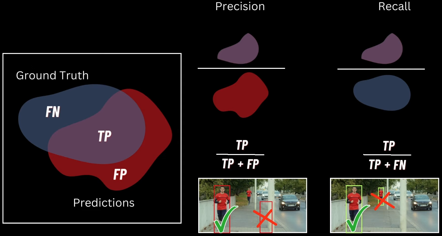 Give a set of predictions by a model of the "person class" and we also have ground truth predictions of "person class". when we plot these two things in `Venn diagram` we get three things 1. `True Positive` - Overlap between Predictions and Ground truth, here the model prediction is correct 2. `False Positive` - Wrong areas the model predicted which are not in ground truth 3. `False Negetive` - Bounding boxes that model didn't predict. The area apart from the two above Ideally we want both Prediction and Recall to be high - If we have high precision and low recall, then we get the correctly predicted objects but we will miss a lot of valid objects - If we have low precision and high recall, then we get a lot of results, and also get a lot of false positives ##### Average Precision (AP) It is the primary metric for evaluating object detection models, measuring both localization accuracy (via IOU) and classification confidence across all recall levels To understand this we need to understand the _Precision Recall Curve_, It's a graph that plots _Recall as X-Axis_ and _Precision as Y-Axis_ for Different Confidence Thresholds Here Average Precision is the area under the Precision-Recall curve. for each class we follow the following algorithm 1. Sort detections by confidence score (taken from ground truth data) 2. Calculate precision and recall at each confidence threshold 3. Plot the PR curve 4. Compute AP as the area under this curve (interpolated or using 11-point sampling) The formula represents a weighted mean of precisions at each threshold, using the recall increase as the weight. Values range from 0 to 1, where AP = 1.0 indicates perfect detection ##### Mean Average Precision (mAP) mAP is simply the arithmetic mean of AP scores across all object classes. For example, if your model achieves AP of 0.827 for cars, 0.679 for motorcycles, and 0.982 for bicycles, mAP = (0.827 + 0.679 + 0.982) / 3 = 0.829 There are two kind of notations to represent mAP: - `mAP@0.5`: Uses IOU threshold of 0.5 to determine true positives, the PASCAL VOC standard - `mAP@0.5:0.05:0.95`: COCO metric averaging mAP across IOU thresholds from 0.5 to 0.95 in 0.05 increments. This is significantly harder and more discriminative, penalizes loose bounding boxes Here is an example of calculating mAP, for car and human class ![[Pasted image 20251115143039.png]] - `GT Boxes`: 5 ground truth objects - 1 person in red, 4 people in the group (with checkmarks), plus 2 cars - `Prediction Boxes`: Model detections with confidence scores: 0.9, 0.8, 0.78, 0.92 (cars), 0.72, 0.83, 0.91, 0.77 (people), and 0.85, 0.65 (cars) The table shows `cumulative metrics` as you decrease the confidence threshold from 0.91 → 0.72(sorted):​ 1. `Pred/GT Comparison`(predicted images): List of each predicted bounding box (often sorted by confidence score). Beside each, you compare it to each ground truth (GT) object. This comparison asks: Is the prediction a True Positive (TP) or a False Positive (FP)? - `TP`: Prediction matches a GT box and passes the IOU threshold (e.g., IOU > 0.5) - `FP`: Prediction does not sufficiently match any remaining GT, or is a duplicate detection 2. `TP/FP Indicator`: The next column is an explicit label, either TP (1) or FP (0), for each prediction after comparing with GT 3. `Cumulative TP`: As you move down the predictions (from highest to lowest confidence), this column tallies how many TPs have been found so far 4. `Cumulative FP`: This column counts total FPs discovered so far as you add each prediction 5. `Precision`:

\text{Precision} = \frac{\text{Cumulative TP}}{\text{Cumulative TP} + \text{Cumulative FP}}

$$Thistellsus,ateachpredictionthreshold,theproportionofpredictionssofarthatarecorrect6.‘Recall‘:$$

\text{Recall} = \frac{\text{Cumulative TP}}{\text{Total\ Ground\ Truth\ (GT)}}

This shows, at each step, what fraction of all GT objects have been detected so far After we get the AP for each class we plot it on the graph and the average of area under the plots of the graphs of different classes is Mean Average Precision(mAP). Also the actual computation of AP can be done using multiple by using multiple approaches, here are two of them - `Area under Curve` (AUC): - Precision Recall curve as a series of steps, at each distinct recall level, draw a rectangle whose height is the precision at that point - The area is the sum of the heights of all these rectangles, each weighted by how much recall increased at that step: $$ AP = \sum_{i=1}^{n} (r_i - r_{i-1}) \cdot p_i

    Where `pi` and `ri` are the precision and recall at the `i-th` threshold​
- This approach is used by scikit-learn and COCO mAP standards; it's direct and reflects the empirical performance across all recall levels

• Interpolation Methods:
  • Instead of just using the raw precision at each recall point, 11-point interpolation (PASCAL VOC, classic method) records precision at 11 recall levels (0, 0.1, … 1.0)
  • At each recall value, take the highest precision found for that or any higher recall threshold:

$$\text{InterpolatedPrecision}(r)=\underset{\hat{r}\ge r}{\max }\text{Precision}(\hat{r})$$

- AP is then averaged over these values:    
$$

AP = \frac{1}{11} \sum_{r \in {0, 0.1, \ldots, 1.0}} \text{InterpolatedPrecision}(r)

- This makes the curve "flat" between points, which can slightly inflate scores for models with irregular curves Code for calculating area for Precision Recall graph for a set of classes using both the methods(AUC and Interpolation) ```python def compute_map(det_boxes, gt_boxes, iou_threshold=0.5, method='area'): # Collect all ground-truth class labels gt_labels = {cls_key for im_gt in gt_boxes for cls_key in im_gt.keys()} aps = [] for label in gt_labels: print(f"Computing AP for {label}") # Collect all detections for this class cls_dets = [ [im_idx, det] for im_idx, im_dets in enumerate(det_boxes) for det in im_dets.get(label, []) ] # Sort by confidence (descending) cls_dets = sorted(cls_dets, key=lambda k: -k[1][-1]) # Track matched GT boxes gt_matched = [ [False] * len(im_gts.get(label, [])) for im_gts in gt_boxes ] # Total GT count for this class num_gts = sum(len(im_gts.get(label, [])) for im_gts in gt_boxes) tp = [0] * len(cls_dets) fp = [0] * len(cls_dets) # Loop over detections for det_idx, (im_idx, det_pred) in enumerate(cls_dets): im_gts = gt_boxes[im_idx].get(label, []) max_iou_found = -1 max_iou_gt_idx = -1 # Find best match GT box for gt_idx, gt_box in enumerate(im_gts): iou = get_iou(det_pred[:-1], gt_box) if iou > max_iou_found: max_iou_found = iou max_iou_gt_idx = gt_idx # Apply matching rules if ( max_iou_found < iou_threshold or max_iou_gt_idx == -1 or gt_matched[im_idx][max_iou_gt_idx] ): fp[det_idx] = 1 else: tp[det_idx] = 1 gt_matched[im_idx][max_iou_gt_idx] = True # Accumulate TP, FP tp = np.cumsum(tp) fp = np.cumsum(fp) eps = np.finfo(np.float32).eps recalls = tp / np.maximum(num_gts, eps) precisions = tp / np.maximum((tp + fp), eps) # ----------------------------- # AREA METHOD (Pascal VOC 2010+) # ----------------------------- if method == "area": recalls = np.concatenate(([0.0], recalls, [1.0])) precisions = np.concatenate(([0.0], precisions, [0.0])) # Precision envelope for i in range(len(precisions) - 1, 0, -1): precisions[i - 1] = np.maximum(precisions[i - 1], precisions[i]) # Points where recall changes i = np.where(recalls[1:] != recalls[:-1])[0] # Actual AP = sum over recall steps ap = np.sum((recalls[i + 1] - recalls[i]) * precisions[i + 1]) # ----------------------------- # 11-POINT INTERPOLATED METHOD # ----------------------------- elif method == "interp": ap = 0.0 for interp_r in np.arange(0, 1.0001, 0.1): precision_at_r = precisions[recalls >= interp_r] max_prec = precision_at_r.max() if precision_at_r.size > 0 else 0.0 ap += max_prec ap /= 11.0 else: raise ValueError("Method can only be 'area' or 'interp'") print(f"AP for class {label} with threshold {iou_threshold:.2f} = {ap:.4f}") # compute for all classes and append them aps.append(ap) mean_ap = sum(aps) / len(aps) return mean_ap ``` ##### ROI(Region of Interest) Pooling Layer ROI Pooling is the layer in Fast R‑CNN that converts variable‑size region proposals into fixed H×W features by max‑pooling bins from a shared convolutional feature map, enabling a single conv pass per image and per‑ROI fully connected heads for classification and box regression. It exists to make detection fast and end‑to‑end by avoiding thousands of conv forward passes while still feeding fixed‑size vectors to FC layers - Runs the backbone CNN once per image, then slices features per proposal, which cuts inference from seconds to sub‑second on VOC - Produces fixed‑size tensors for each ROI so FC classification and bounding box regression heads can be shared across proposals of different original sizes How it works ? - Inputs: a conv feature map and a set of ROIs defined in image coordinates, plus the backbone’s stride to map those ROIs into feature‑map coordinates - Quantize the mapped ROI coordinates to integers (rounding) so they index discrete feature‑map cells; this may include some pixels outside the ROI and exclude some inside due to rounding - Divide the quantized ROI window into an H×W grid of bins (e.g., 7×7), and in each bin take channel‑wise max pooling to produce a fixed H×W×C output per ROI that is then flattened for the heads - Example mapping: a 400×400 image with stride 40 yields a 10×10 feature map; an ROI mapped to non‑integer cell boundaries is rounded, then split into equal bins like 2×2 or 7×7 before per‑bin max pooling Given an ROI on the feature map with top-left coordinate (x, y), height (roi_{height}), and width (roi_{width}), ROI pooling divides this window into (pool_h) rows and (pool_w) columns (e.g., 7 x 7) Vertical bin boundaries:

h_{\text{start}} = \left\lfloor \frac{j \cdot roi_{height}}{pool_h} \right\rfloor

h_{\text{end}} = \left\lceil \frac{(j+1) \cdot roi_{height}}{pool_h} \right\rceil

$$Horizontalbinboundaries:$$

w_{\text{start}} = \left\lfloor \frac{i \cdot roi_{width}}{pool_w} \right\rfloor

w_{\text{end}} = \left\lceil \frac{(i+1) \cdot roi_{width}}{pool_w} \right\rceil

$$PoolingOperation:Eachbin(i,j)ismax-pooledindependentlyforeachchannelThefinalROIpooledoutputisafixed-sizetensor:$$

(pool_h,; pool_w,; C)

even though the original ROI may have any spatial size ##### RPN(Region Proposal Network) The job of RPN is to return the regions which possibly contain the objects we need, to do this, we take the input image, pass it through a CNN that outputs the feature map, and we perform the Sliding window operation on this feature map and predict the object in the window is correct or not. And with also the parameter sharing of the CNN, this operation is not that costly But there is a problem, as we're taking a sliding window of fixed size and the target objects will not be in fixed sizes, thus we use _Anchor Boxes_, now at a given location we make multiple predictions using multiple boxes of different sizes and make the predictions But there is a problem here, like when we use boxes of different size there is a low chance, that the object we want will fit into that box, so to handle this case, we predict the part of the object, for example, if the box have only tire of the car, we still take it as yes, as we're predicting the part of the expected object car, these will be enlarged and get clear object in the Bounding Box Regressor(discussed above) layer that comes later ![[Pasted image 20251119170320.png]] After passing these Anchor boxes in the activation function(a mathematical function in a neural network that determines a neuron's output by introducing non-linearity to the weighted sum of its inputs), we use 1x1 convolution on this to generate a prediction, and for this we use two such convolution layers 1. One have output channel of 2k, which are meant to be the foreground and background score prediction for each of the anchor boxes at each window location. so two predictions at k anchor boxes at each location, here we implement objectness as a two class SoftMax layer hence 2k 2. The other 1x1 convolution is of 4k channels, these are the four transformation parameters that the network predicts, basically the transformation that each of those K reference boxes must undergo to better fit the underlying object and in the same like objectness we will have 4k values for each location of the feature map ![[Pasted image 20251119170910.png]] Now when we put two architectures together, we can see the flow Input Image passed through CNN -> Feature maps generated and given to RPN -> The generated selective proposals are pass to the detection specific part of the network which using ROI pooling on the feature maps produces detection predictions for the proposals that were generated by RPN ![[Pasted image 20251119172118.png]] In the training part of the anchor boxes we use [[13. Object Detection#iou-intersection-over-union|IOU]] to select the best answer from proposed boxes ![[Pasted image 20251119172724.png]] _RPN Training_: RPN generates ~20,000 anchor boxes across the image (for 1000×600 image with stride 16, 9 anchors per location). Each anchor needs a ground truth label Assignment rules: 1. Positive anchors (foreground): - IOU with any ground truth box > 0.7 - OR anchor with highest IOU with a ground truth box (even if < 0.7). This rule ensures every ground truth object has at least one positive anchor, preventing training samples where no anchor matches small/oddly-shaped objects 2. Negative anchors (background): - IOU with all ground truth boxes < 0.3 3. Ignored anchors: - 0.3 ≤ IOU ≤ 0.7 - These are not used in training (neither positive nor negative) This creates a clear separation: high overlap = object, low overlap = background. The middle zone is ambiguous and excluded Mini-batch Sampling: From all positive and negative anchors: - Sample N images (typically N=1 in the video) - From each image, sample 256 anchors total: - 128 positive (foreground) - 128 negative (background) - If fewer than 128 positives exist, pad with negatives to reach 256 total This 1:1 ratio prevents class imbalance (background anchors vastly outnumber foreground) RPN Loss Function:

\mathcal{L} = \frac{1}{N_{\text{cls}}} \sum_i L_{\text{cls}}(p_i, p_i^) ;+; \lambda , \frac{1}{N_{\text{reg}}} \sum_i p_i^ , L_{\text{reg}}(t_i, t_i^*)

$$Notation:-i:anchorindex-p_i:predictedprobabilitytheanchorisforeground(2-classSoftMax)-p_i^{\ast }:groundtruthlabel(1=foreground,0=background)-t_i=(t_x,t_y,t_w,t_h):predictedboxregressionoffsets-t_i^{\ast }=(t_x^{\ast },t_y^{\ast },t_w^{\ast },t_h^{\ast }):groundtruthboxregressionoffsets-N_{c}ls=256:numberofsampledanchors-N_{r}eg=2400:numberofanchorlocations-\lambda =10:balancingweight-ClassificationLoss:$$

L_{\text{cls}}(p_i, p_i^*) = -\log(p_{i,\text{correct}})

$$Cross-entropyoverall256sampledanchors(bothpositiveandnegative)-RegressionLoss:$$

L_{\text{reg}}(t_i, t_i^) = \sum_{j \in {x, y, w, h}} \text{SmoothL1}(t_{i,j} - t_{i,j}^)

$$-SmoothL1function:$$

\text{SmoothL1}(x) = \begin{cases} 0.5x^2, & |x| < 1 \ |x| - 0.5, & \text{otherwise} \end{cases}

$$-Theregressionlossisappliedonlyforpositiveanchors:$$

p_i^* = 1 \quad \Rightarrow \quad \text{apply reg loss}

$$If(p_i^{\ast }=0),regressionisignoredTargetTransformationComputation:Given:-Anchorbox:x_a,y_a,w_a,h_a-Groundtruthbox:x_{gt},y_{gt},w_{gt},h_{gt}$$

t_x^* = \frac{x_{gt} - x_a}{w_a}, \quad t_y^* = \frac{y_{gt} - y_a}{h_a}

t_w^* = \log\left(\frac{w_{gt}}{w_a}\right), \quad t_h^* = \log\left(\frac{h_{gt}}{h_a}\right)

$$Inversetransform(usedduringinference):$$

x’ = t_x \cdot w_a + x_a, \quad y’ = t_y \cdot h_a + y_a

w’ = w_a \cdot e^{t_w}, \quad h’ = h_a \cdot e^{t_h}

$$Thisformulationprovidesscale-invariantregressionthroughtheuseoflog-spacewidth/heigh{t}_{F}astR-CNNDetectionHeadTrainin{g}_{:}OnceRPNgeneratesproposals,thedetectionhead(FastR-CNNpart)istrainedFromRPN-generatedproposals(afterNMS,top-2000duringtraining):Foregroundproposals:-IOU>0.5withanygroundtruthbox-Assignedclass=classofGTboxwithhighestIOUBackgroundproposals:-0.1\le IOU<0.5withanyGTbox-Assignedclass=0(background)Ignored:-IOU<0.1(notsampled)Mini-batchSamplingforDetection:-SampleN=2imagesperbatch-Fromeachimage,sampleR/N=64/2=32proposals-Totalbatchsize:64proposals-Maintain25Soperbatch:16foreground,48backgroundproposalsDetectionLoss(FastR-CNN):$$

\mathcal{L}(p, u, t^{u}, v)

L_{\text{cls}}(p, u) + \lambda ,[u \ge 1] , L_{\text{loc}}(t^{u}, v)

$$Notation:-p=(p_0,p_1,...,p_K):predictedclassprobabilities-u:groundtruthclass-(u=0)\to background-(u=\mathrm{1...}K)\to objectclasses-t^u:predictedboxdeltasforclass(u)(from4Koutputs,choosethe4correspondingtoclass(u))-v:groundtruthboxregressiontargetClassificationLoss:$$

L_{\text{cls}}(p, u) = -\log(p_u)

$$Localization(BoundingBoxRegression):$$

L_{\text{loc}}(t^{u}, v)

\sum_{i \in {x, y, w, h}} \text{SmoothL1}(t^{u}_i - v_i)

$$SmoothL1definition(forreference):$$

\text{SmoothL1}(x) = \begin{cases} 0.5x^2, & |x| < 1 \ |x| - 0.5, & \text{otherwise} \end{cases}

$$Regressionappliesonlytoforegroundclasses:$$

[u \ge 1] = \begin{cases} 1, & u > 0 \ 0, & u = 0 \end{cases}

_Joint Training Strategy_: - Forward Pass Flow 1. Shared conv layers: Image → feature map (one pass) 2. RPN branch: - 3×3 conv → 1×1 conv (objectness + box deltas) - Generate ~20,000 anchor predictions - Apply NMS, select top-2000 proposals 3. Detection branch: - ROI pooling on top-2000 proposals using shared feature map - FC layers → classification (K+1) + regression (4K) Loss Computation: For RPN: - Sample 256 anchors (128 pos, 128 neg) - Compute RPN loss: L_rpn For Detection: - Sample 64 proposals from RPN output (16 pos, 48 neg) - Compute detection loss: L_det Total loss: L_total = L_rpn + L_det Backward Pass: - RPN-specific layers: gradients from L_rpn - Detection-specific layers: gradients from L_det - Shared conv layers: gradients from both L_rpn and L_det This joint optimization teaches shared features useful for both proposal generation and object classification _4-Step Alternating Training_ - Step 1: Train RPN - Initialize from ImageNet pretrained model - Train RPN layers only (conv layers also fine-tuned) - Use RPN loss with anchor assignments - Output: RPN weights W_rpn(1) - Step 2: Train Fast R-CNN (Separate Network) - Initialize separate Fast R-CNN from ImageNet - Generate proposals using RPN from Step 1 - Train detection layers on these proposals - Output: Detection weights W_det(2) (including separate conv layers) At this stage, RPN and Fast R-CNN have separate conv layers (no sharing yet). This is the "unshared" baseline - Step 3: Fine-tune RPN (Shared Conv) - Take conv layers from Step 2's Fast R-CNN (detection-tuned) - Initialize RPN with these shared conv layers - Freeze conv layers, fine-tune only RPN-specific layers (3×3, 1×1 conv) - Output: RPN weights WRPN(3)W_{RPN}^{(3)}WRPN(3) with shared conv - Step 4: Fine-tune Fast R-CNN (Shared Conv) - Keep shared conv layers from Step 3 frozen - Generate proposals using RPN from Step 3 - Fine-tune only detection-specific layers (FC, classification, regression heads) - Output: Final Faster R-CNN model Result: Shared conv layers + RPN layers + detection layers all trained, but in alternating fashion _Summary_: - RPN training: 256 anchors per batch (50% pos), IoU thresholds 0.7/0.3, loss has cls + reg with λ=10 - Detection training: 64 proposals per batch (25% pos), IoU thresholds 0.5/0.1, loss has cls + reg with λ=1 - 4-step alternating: Train RPN → train detection (separate) → fine-tune RPN (shared conv, frozen) → fine-tune detection (shared conv, frozen) - Why it works: Shared conv layers learn features useful for both objectness (RPN) and classification (detection). Two-stage refinement (anchor → proposal → detection box) is superior to one-stage ##### DETR(Detection Transformer) It's a transformer based object detection model. This model will be given input as image and the output will be bounding boxes wrt class predictions and there confidence scores _Overview_: 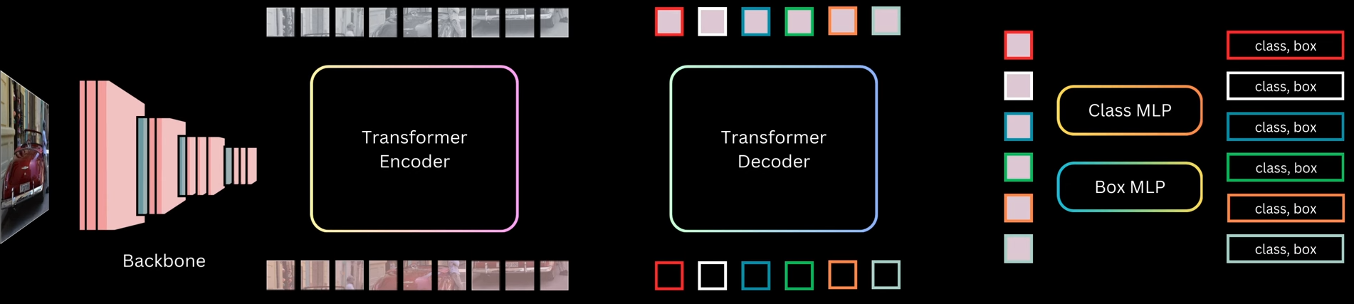 1. The input image is first passed through a backbone, which is a pre-trained CNN like ResNet-50 or ResNet-101 (trained on ImageNet). The last pooling and classification layers are removed to get a feature map that captures semantic information from different image regions. These grid cells are flattened into a sequence and passed to a transformer encoder 2. The encoder is made of multiple self-attention and feed-forward layers with residual connections. After encoding, each grid cell representation contains contextual information from the whole image 3. The decoder takes a fixed number of object queries as input. These object queries are just randomly initialized embeddings. The decoder refines these query embeddings and turns each one into an object prediction. Each query predicts exactly one bounding box and one class, so the number of predictions equals the number of queries 4. The transformer decoder layers are similar to encoder layers but also include cross-attention, where query embeddings attend to the encoder’s image features. After all decoder layers, the final query representations are passed through two MLPs to predict class labels and bounding boxes. Some queries predict actual objects like cars or persons, while the remaining ones predict the background class 5. Since there are as many predictions as queries, the key question during training is how to assign ground-truth targets to these predictions ? Unlike anchor-based models like Faster R-CNN or SSD, DETR does not rely on anchor overlap. Instead, it evaluates predictions using a cost based on class probability and box distance (including IOU-based measures) 6. In anchor-based models, multiple anchors can match the same target, leading to duplicate predictions and the need for NMS. DETR enforces a one-to-one mapping: each target box is matched to only one predicted box, and unmatched predictions are assigned the background class 7. This one-to-one mapping reduces duplicate boxes and encourages each query to predict a different object or background if no object exists 8. DETR treats object detection as a set prediction problem. The model predicts a set of boxes, and a matching algorithm assigns predictions to ground-truth boxes uniquely and optimally. Each possible prediction-target pair has a matching cost, computed using box distance and class probability distance. The exact cost calculation is not important here, just that lower cost means a better match 9. Among all valid one-to-one assignments, DETR selects the assignment with the minimum total cost. Predictions not matched to any target are treated as background 10. During training, matched predictions learn to predict the correct class and box coordinates, while unmatched predictions learn to predict the background class 11. Conceptually, this is similar to earlier models where predictions are mapped to targets or background. The main difference is that DETR changes the matching strategy and removes anchors and NMS entirely _Backbone_: 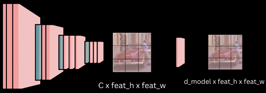 - DETR uses a pre-trained CNN backbone, usually ResNet-50 or ResNet-101, which is first trained on the ImageNet classification task - To use it as a feature extractor, the final pooling and fully connected layers are removed. This gives a feature map of size `C × feat_h × feat_w`, where `C` is the number of output channels from the last convolution layer. Since the overall stride is 32, an input image of size `640 × 640` produces a feature map of size `20 × 20` - To match the transformer’s hidden dimension, a projection layer is added. This is a `1 × 1` convolution that converts the backbone output channels to the transformer dimension - After this projection, the final feature map has shape `D_model × feat_h × feat_w`, where `D_model` is the transformer hidden size _DETR Encoder_: 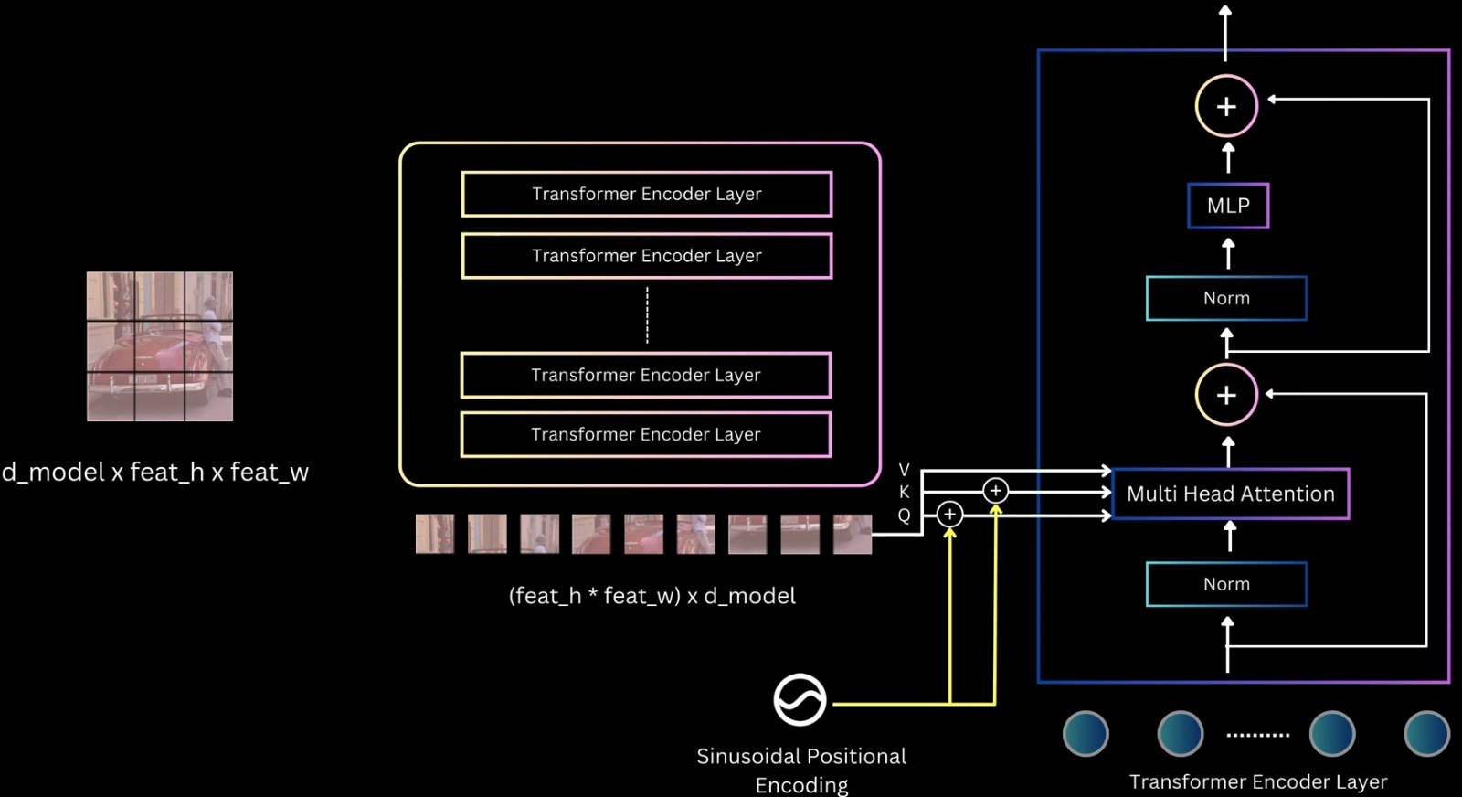 - The transformer encoder takes a sequence as input. So the backbone feature map of shape `D_model × feat_h × feat_w` is flattened by collapsing the spatial dimensions, giving a sequence of length `feat_h × feat_w`, where each element is a `D_model`-dimensional feature vector - This sequence is passed to the encoder, which is a stack of transformer encoder layers. The input to the first encoder layer is the projected backbone features, and for the remaining layers, the input is the output of the previous encoder layer - Each encoder layer follows the standard transformer structure: - Layer normalization - Self-attention - Residual connection - Layer normalization - Feed-forward MLP - Residual connection - The encoder operates on the sequence in a permutation-invariant way, so it needs spatial information. To handle this, 2D positional encodings are added - DETR uses sinusoidal positional encoding, extended to 2D. A `D/2`-dimensional encoding is created for the height coordinate and another `D/2`-dimensional encoding for the width coordinate, and they are concatenated to form a `D_model`-dimensional positional encoding for each spatial location - Unlike standard transformers where positional encoding is added only at the input, DETR adds positional information at every self-attention layer, specifically to the query and key tensors. The authors found this gives slightly better results - Through self-attention, the encoder allows any part of the image to attend to any other part. This helps in understanding the full extent of objects and in capturing contextual information. The final output of the encoder is a sequence with the same shape as the input, but with features that are more suitable for the object detection task _DETR Decoder_: - The decoder is made of a stack of decoder layers. The first decoder layer takes the object queries as input, and each following layer takes the output of the previous decoder layer. Each decoder layer contains: - Layer normalization - Self-attention - Residual connection - Layer normalization - Cross-attention - Residual connection - Layer normalization - Feed-forward MLP - Residual connection - `Multi Head Attention(MHA)` - 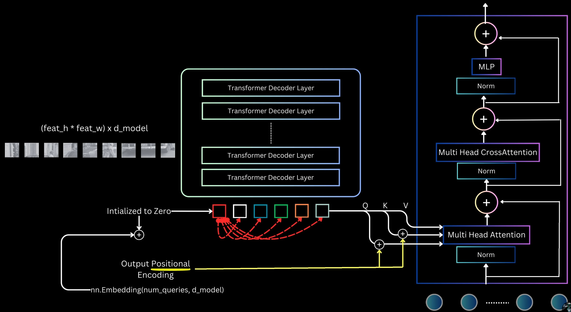 - In the self-attention block, each object query attends to all other queries. This allows the model to reason about relationships between different objects, such as relative positions or co-occurrence - For self-attention, Q, K, and V are all derived from the object queries - Instead of initializing queries as random embeddings, DETR initializes all queries as zeros - A set of learnable embeddings, called output position encodings, is added to the query slots only inside the attention layers before computing Q and K. These embeddings do not represent spatial position. The name is borrowed from language models and can be confusing - All query slots start identical, and the only thing that differentiates them during attention is these output position embeddings - This design is similar to the encoder, where spatial position information is added only at the attention layers rather than at the input - `Multi Head Cross-Attention (MHCA)` - 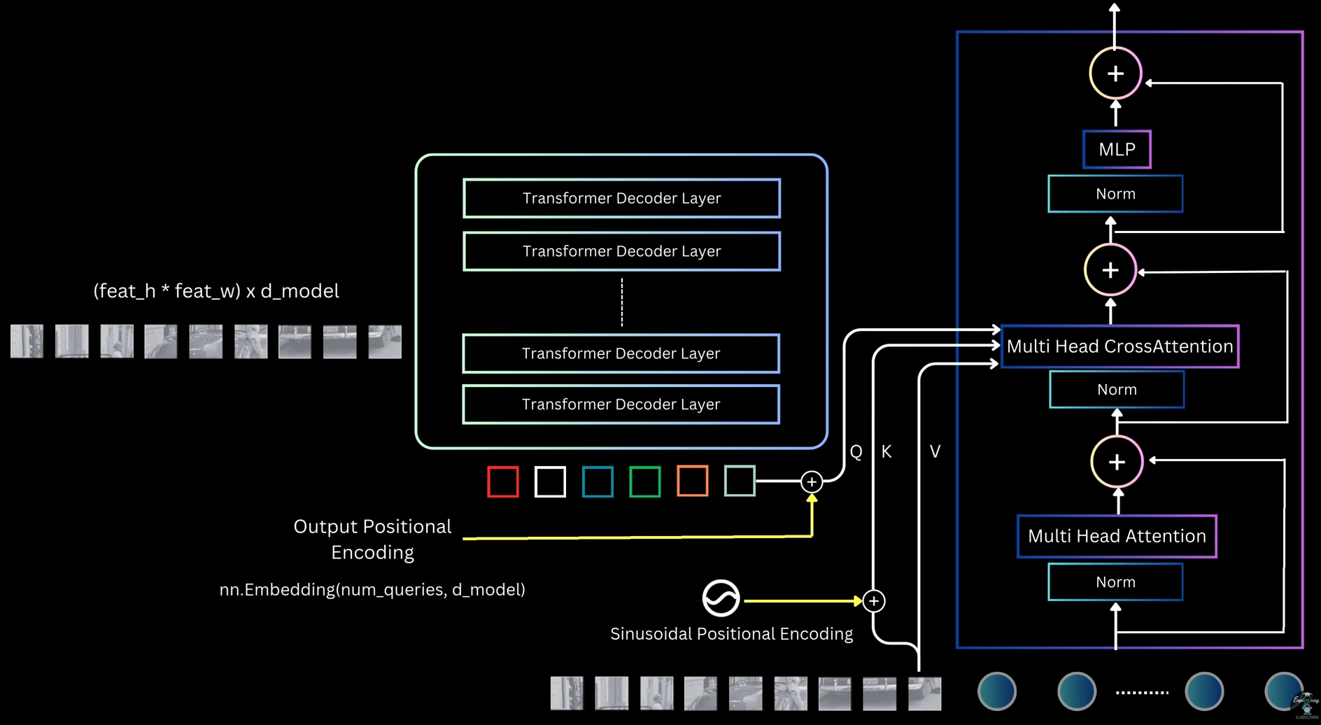 - The cross-attention layer allows object queries to attend to image features from the encoder, giving them access to the full image context - In cross-attention: - Q comes from the query slots - K and V come from the encoder output (image features) - Before computing attention: - The 2D sinusoidal positional encoding is added to the encoder image features before computing K - The output position embeddings are added to the query slots before computing Q - This helps the decoder combine object-level reasoning with global and local image information - `Decoder Output`: - After passing through all decoder layers, the decoder outputs n query representations, one for each query slot - Each output query is independently decoded into a prediction using two shared MLPs: - One MLP predicts class probabilities - Another MLP predicts bounding box coordinates `(cx, cy, width, height)` - Box coordinates are normalized between 0 and 1 with respect to the input image - Since all queries are processed in parallel and MLP weights are shared, the model produces n object predictions in parallel, one from each query - After a forward pass, DETR outputs n predicted boxes - During training, each prediction must be assigned a target, which can be a ground-truth box, or background - The key constraint: - Each prediction → only one target - Each target → only one prediction - This is a one-to-one assignment problem, which is solved using the [[13. Object Detection#hungarian-matching-algorithm|Hungarian Matching Algorithm]] _Matching Strategy and Cost of DETR_: Prediction-Target Matching: - Just like the worker-task example, DETR assigns predicted boxes to target boxes - Constraints: - One predicted box → one target - One target → one predicted box - Sometimes: - Number of predicted boxes > number of targets - Number of targets < number of predictions Making the Cost Matrix Square: - To apply Hungarian matching, we need a square cost matrix. - DETR solves this by: - Fixing the number of predictions using a fixed number of object queries - Example: - Max objects per image = 100 - Number of queries = 100 - Model always predicts 100 boxes - If an image has fewer targets: - Extra targets are treated as dummy background boxes - Cost of assigning any prediction to a background box = 0 - This gives a square matrix and allows Hungarian matching - In practice, this dummy background handling is abstracted away by the library Cost Function for Matching: - To apply Hungarian matching, we must define the cost of assigning a predicted box to a target box. - The total cost has two parts: 1. Classification Cost: - We look at the probability predicted by the model for the target class. - Example: - Target class = person - Predicted probability for person = `p_person` - We want: - High probability → low cost - Low probability → high cost $$ \mathcal{L}_{cls} = 1 - p_{\text{target}} $$ - Since adding a constant does not change optimal assignment, we can simplify to: $$ \mathcal{L}_{cls} = - p_{\text{target}} $$ 2. Localization Cost: - Localization cost measures how close the predicted box is to the target box - L1 Distance (Box Regression) - Box format: c_x, c_y, w, h $$ \mathcal{L}_{L1} = \| b - \hat{b} \|_1 $$ - Issue: Same relative error gives different L1 values for small vs large boxes Generalized IOU (GIoU) - To handle scale differences, DETR also uses Generalized IOU - We want: - High overlap → low cost - Low overlap → high cost

\mathcal{L}_{giou} = - \text{GIoU}(b, \hat{b})

$$TotalMatchingCost:Thefinalcostforassigningapredictedboxtoatargetboxisaweightedsum:$$

\mathcal{C}{i,j} = \lambda{cls} \mathcal{L}_{cls}

• \lambda_{L1} \mathcal{L}_{L1}
• \lambda_{giou} \mathcal{L}_{giou}

$$Where:-‘i‘\to predictedboxindex-‘j‘\to targetboxindex-‘\lambda ‘valuesareweightinghyperparameter{s}_{D}ETRLos{s}_{:}-DETRusestheassignmentsproducedbyHungarianmatching-Thelossisacombinationof:1.ClassificationLoss-Forpredictedboxesassignedtoatarget:‘Ground-truthclass=classoftheassignedtargetbox‘-Forunassignedpredictions:‘Ground-truthclass=background‘-Classificationlossiscomputedforallpredictedboxes$$

\mathcal{L}_{cls} = \text{CE}(y_i, \hat{p}_i)

$$-Where:-‘y_i‘=ground-truthclasslabel(includingbackground)-‘p_i‘=predictedclassprobabilities-‘CE‘=cross-entropyloss-Localizationloss-Eachpredictedboxisassignedeither:-aground-truthtargetbox,or-thebackgroundclass2.LocalizationLoss-Localizationlossiscomputedonlyforpredictionsassignedtoanon-backgroundtarget-SmoothL1Loss:-Measureserrorbetweenpredictedandtargetboxcoordinates-Boxformat:‘(c_x,c_y,w,h)‘$$

\mathcal{L}_{L1} = \text{SmoothL1}(b_i, \hat{b}_i)

$$-GeneralizedIOU(GIoU)Loss-Encourageshigheroverlapbetweenpredictedandtargetboxes-DefinedasoneminusGIoU$$

\mathcal{L}_{giou} = 1 - \text{GIoU}(b_i, \hat{b}_i)

$$3.FinalDETRLoss-Thetotallossisaweightedsumofclassificationandlocalizationlosses:$$

\mathcal{L}{DETR} = \lambda{cls} \mathcal{L}_{cls}

• \lambda_{L1} \mathcal{L}_{L1}
• \lambda_{giou} \mathcal{L}_{giou}

- Where: `λ` values control the relative importance of each term - Each predicted box is assigned either: - a ground-truth target box, or - the background class _Auxiliary Losses in DETR_: #Q Why Auxiliary Losses Are Used #A - Using only the final decoder layer can make training slow to converge - To improve convergence and mAP: DETR applies losses at all decoder layers, not just the last one. Auxiliary Loss Mechanism - Each decoder layer outputs object query representations. - These outputs are passed through the same shared MLPs: - One for class prediction - One for bounding box prediction - For each decoder layer: 1. Predicted boxes are generated 2. Hungarian matching is applied independently 3. Classification and localization losses are computed Auxiliary Loss Formula - If there are `L` decoder layers:

\mathcal{L}{aux} = \sum{l=1}^{L} \left( \lambda_{cls} \mathcal{L}_{cls}^{(l)}

• \lambda_{L1} \mathcal{L}_{L1}^{(l)}
• \lambda_{giou} \mathcal{L}_{giou}^{(l)} \right)

$$-TotalTrainingLoss$$

\mathcal{L}{total} = \mathcal{L}{DETR}^{(final)}

• \mathcal{L}_{aux}

- Training: - Uses losses from all decoder layers - Helps earlier layers learn meaningful representations - Inference: - Uses only the final decoder layer outputs - Earlier layer outputs are ignored _Connecting the Dots_: - Hungarian matching → assigns predictions to targets - DETR loss → trains predictions using those assignments - Auxiliary loss → stabilizes training and improves convergence - No anchors, no NMS, clean one-to-one prediction setup ##### Hungarian Matching Algorithm _Intuition_: Worker - Task Problem - Imagine n workers and n tasks - Every worker can do every task, but with different costs - Each worker can do only one task, and each task can be assigned to only one worker - Cost Matrix - Rows → workers - Columns → tasks - Values → cost ``` Task1 Task2 Task3 Task4 WorkerA 10 7 8 2 WorkerB 6 4 5 3 WorkerC 7 6 9 5 WorkerD 8 5 6 4 ``` - Goal: assign tasks to workers with minimum total cost - This is exactly the same as assigning predicted boxes to target boxes in DETR - Key Idea Behind the Algorithm: - Adding or subtracting a constant value from a row or column: - Changes the total cost - Does NOT change the optimal assignment - The algorithm uses this idea to create zeros in the matrix - A zero cost means a very good assignment _Hungarian Algorithm_ - Step 1: Row Reduction - Subtract the minimum value in each row from all elements of that row - Example (Row A minimum = 2): - Before: 10 7 8 2 - After : 8 5 6 0 - This keeps the optimal assignment unchanged - Goal: introduce zeros - Step 2: Column Reduction - Subtract the minimum value in each column from all elements of that column - After row + column reduction, we may get something like: ``` T1 T2 T3 T4 A 8 4 6 0 B 0 3 5 2 C 0 7 1 7 D 2 0 0 1 ``` - Step 3: Cover All Zeros with Minimum Lines - Draw the minimum number of horizontal and vertical lines needed to cover all zeros ``` T1 T2 T3 T4 A 8 4 6 0 ← line B 0 3 5 2 C 0 7 1 7 D 2 0 0 1 ← line ↑ ↑ line line ``` - Count the number of lines used - Step 4: Check for Solution - If number of lines = n, then: - A zero-cost assignment exists - We are done - If number of lines < n, then: - We need to create more zeros - In this example: - Lines used = 3, Required = 4 - Thus not done yet - Step 5: Find Minimum Uncovered Value - Look at all entries not crossed by any line - Find the smallest value among them - Uncovered region (example): - 1, 2, 3 ... - Minimum = 1 - Step 6: Update the Matrix - Subtract this minimum value from: all uncovered elements - Add the same value to: elements covered twice (intersection of two lines) - This operation: - Creates new zeros - Keeps all values non-negative - Preserves the optimal assignment - Step 7: Repeat - Go back to Step 3 - Repeat until: number of covering lines = n - Eventually we get: ``` T1 T2 T3 T4 A 8 4 6 0 B 0 3 5 2 C 2 7 0 6 D 2 0 1 0 ``` - Now we can assign: A → T4, B → T1, C → T3, D → T2 - 4 zero-cost assignments _Connection to [[13. Object Detection#detrdetection-transformer|DETR]]_: - Rows → predicted boxes - Columns → ground-truth boxes - Cost → combination of: - class probability loss - bounding box distance loss - Hungarian matching ensures: - one-to-one mapping - no duplicate predictions - no need for NMS