CUDA

This is what massively parallel computing looks like. And let us understand how this is 50 - 100x faster than the CPU

__global__ void matmul_tiled(float* C, const float* A, const float* B, int M, int N, int K) {
    __shared__ float a_tile[16][16];  // Fast shared memory
    __shared__ float b_tile[16][16];
 
    int tx = threadIdx.x, ty = threadIdx.y;
    int row = blockIdx.y * 16 + ty;
    int col = blockIdx.x * 16 + tx;
    float sum = 0.0f;
 
    // Process tiles cooperatively across thousands of threads
    for (int phase = 0; phase < (K + 15) / 16; ++phase) {
        a_tile[ty][tx] = A[row * K + phase * 16 + tx];
        b_tile[ty][tx] = B[(phase * 16 + ty) * N + col];
        __syncthreads();  // Coordinate 256 threads at once
 
        for (int i = 0; i < 16; ++i)
            sum += a_tile[ty][i] * b_tile[i][tx];
        __syncthreads();
    }
 
    C[row * N + col] = sum;
}

The Problem: The Computational Bottleneck Consider the task of multiplying two matrices, A and B, to produce a third matrix, C C = A * B For each element C[i,j] in the output matrix, we must compute a dot product of a row from A and a column from B. The formula is: C[i, j] = Σ (A[i, k] * B[k, j]) for all k A standard single-threaded CPU computes each of these dot products one by one. If A and B are 1000x1000 matrices, this requires 1 billion multiplications and 1 billion additions. This is computationally expensive and slow

Scale of the Performance Gap:

• CPU (single-threaded): ~0.5 GFLOPS - computes one element at a time
• CPU (multi-threaded, 16 cores): ~8 GFLOPS - limited parallelism
• GPU (naive CUDA): ~15 GFLOPS - thousands of threads, but memory-bound
• GPU (optimized CUDA): ~800+ GFLOPS - efficient memory usage
• GPU (highly-tuned libraries): ~20,000+ GFLOPS - professional optimization

The Solution: Massive Parallelism The key observation is that the calculation for each element C[i,j] is completely independent of the calculation for any other element C[x,y]. We don’t need to compute C[0,0] before we compute C[5,5]. We can, in theory, compute all of them simultaneously. This is where the GPU excels. A modern GPU contains thousands of simple processing cores designed to execute the same instruction on different data in parallel

Our strategy will be:

1. Launch a Grid of Threads: Assign one GPU thread to be responsible for calculating a single element of the output matrix C
2. Distribute the Work: Each thread will use its unique ID to identify which row i from matrix A and which column j from matrix B it needs to process
3. Execute in Parallel: All threads will perform the dot product calculation Σ (A[i, k] * B[k, j]) at the same time
4. Optimize: We will then identify performance bottlenecks related to memory access and introduce an optimization using tiled matrix multiplication with shared memory

GPU Architecture

• A CPU is like a single, master chef. This chef is incredibly skilled and can perform any complex cooking task (like a difficult multi-step sauce) very quickly and efficiently, one task at a time
• A GPU is like a massive commercial kitchen staffed with thousands of junior chefs. Each junior chef can only perform simple, repetitive tasks (like chopping a single vegetable). While any individual junior chef is much slower and less versatile than the master chef, they can all chop vegetables simultaneously. If you need to chop 10,000 carrots, the army of junior chefs will finish the job orders of magnitude faster than the single master chef

Real Hardware Numbers (NVIDIA RTX 3090 example):

• 10,496 CUDA cores (the “junior chefs”)
• 82 Streaming Multiprocessors (the “cooking stations”)
• Each SM can manage up to 2,048 threads concurrently
• Maximum concurrent threads: ~170,000 threads simultaneously
• 24 GB global memory (the “main pantry”)
• 128 KB shared memory per SM (the “workbench per station”)

CUDA programming is the art of breaking down a large problem into thousands of simple, identical tasks that can be assigned to these junior chefs
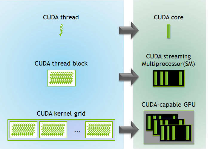
To manage our “army of chefs,” CUDA imposes a three-level hierarchy. This is how we organize the parallel work

1. Thread: The most basic unit of execution. A single “junior chef” that executes a piece of code called a kernel
2. Block: A group of threads. The “chefs” within a single block can cooperate and communicate with each other using a fast, shared workspace. A block is a team of chefs working together at one station
3. Grid: A collection of blocks. The entire “kitchen” is a grid of all the cooking stations (blocks)

When you run a program on the GPU, you launch a kernel function with a specific grid and block structure

This is a 2D Grid of Blocks, and each Block is a 3D arrangement of Threads

Image description:
A large rectangle represents the 'Grid'.
This Grid is tiled with smaller rectangles, each representing a 'Block'. For example, Grid(0,0), Grid(0,1), Grid(1,0), Grid(1,1).
Zoom into one 'Block'. This block is a 3D cube filled with small dots, where each dot is a 'Thread'. For example, Thread(0,0,0), Thread(0,0,1), etc.
Arrow from Grid -> Block -> Thread illustrates the hierarchy.

Hardware Model(Simplified)

Mapping programming hierarchy onto the physical GPU hardware

• Host & Device: In CUDA terminology, the Host is the CPU and its memory (RAM). The Device is the GPU and its memory (VRAM). Your main program runs on the host, and it launches kernels on the device
• Streaming Multiprocessor (SM): The GPU is composed of several Streaming Multiprocessors. Think of an SM as a fully-equipped cooking station in our kitchen analogy. An SM is responsible for scheduling and executing entire blocks of threads
• CUDA Cores: Each SM contains numerous CUDA cores, the actual “junior chefs.” These are the simple processing units that execute the instructions for the threads
• Memory Hierarchy: This is one of the most critical concepts for performance
  • Global Memory: This is the large, primary memory of the GPU (VRAM). It is accessible by all threads from all blocks. However, it is relatively slow. Think of it as the main, large pantry in the kitchen. Any chef can access it, but it takes a long walk to get ingredients
  • Shared Memory: Each SM has a small, extremely fast memory space called shared memory. It is only accessible to the threads within the block currently running on that SM. This is like a small, shared workbench or spice rack at a single cooking station. The team of chefs at that station can share ingredients very quickly without walking to the main pantry

Component	Analogy	Scope	Speed (Bandwidth)	Size	Latency
CUDA Core	Junior Chef	Executes thread	-	-	-
SM	Cooking Station	Executes blocks	-	-	-
Global Memory	Main Pantry	All threads in the grid	~10-50 GB/s	8-80 GB (entire GPU)	~400-800 cycles
Shared Memory	Shared Workbench	Threads within a block	~1-10 TB/s (200x faster!)	48-164 KB per SM	~20-30 cycles
Registers	Chef’s hands	Individual thread	~19 TB/s	64 KB per SM	~1 cycle
The goal of many CUDA optimizations, as we will see, is to minimize slow trips to global memory by using fast shared memory as much as possible

Writing CUDA Kernel: A Parallel “Hello, World!”

The goal is to write a complete program that allocates memory on the GPU, executes a simple calculation in parallel, and brings the result back to the CPU Example: Vector Addition The classic “Hello, World!” prints a line of text. A GPU, however, doesn’t directly print to the console. The equivalent introductory program in parallel computing is vector addition The problem is simple: Given two vectors (arrays of numbers), A and B, compute a third vector, C, where each element is the sum of the corresponding elements in A and B C[i] = A[i] + B[i] This operation is “embarrassingly parallel” because the calculation for C[0] is completely independent of the calculation for C[1], C[2], and so on. We can assign one thread to each index i, and all threads can perform their addition simultaneously A complete CUDA program involves both code for the Host (CPU) and code for the Device (GPU)

1. The Device Code: The Kernel

   • This is the function that each of our GPU threads will execute. In CUDA, we define it using the __global__ keyword
     • __global__ void addKernel(int *c, const int *a, const int *b)
       • __global__ tells the compiler this is a kernel function that can be called from the host and will run on the device
       • It takes pointers to arrays in the GPU’s global memory
   • Inside this function, each thread needs to determine which element i it is responsible for. CUDA provides built-in variables for this:
     • threadIdx.x: The thread’s index within its block
     • blockIdx.x: The block’s index within the grid
     • blockDim.x: The number of threads in each block
   • The unique global index i for any thread is calculated with the formula:
     • int i = blockIdx.x * blockDim.x + threadIdx.x;

   // CUDA Kernel function to add the elements of two arrays
   __global__ void addKernel(int *c, const int *a, const int *b)
   {
       int i = blockIdx.x * blockDim.x + threadIdx.x;
       c[i] = a[i] + b[i];
   }

   • Input: Pointers a, b, and c to integer arrays residing in GPU global memory
   • Output: The array c is modified in place on the GPU

2. The Host Code: Managing the Operation

   • The main() function of our program runs on the CPU. Its job is to set up the data, tell the GPU to run the kernel, and then retrieve the results
   1. Allocate Memory on the GPU
      • We need to allocate separate memory on the device for our three vectors. We use cudaMalloc

      // Allocating GPU Memory
      int *dev_a = 0;
      int *dev_b = 0;
      int *dev_c = 0;
       
      // Allocate memory on the GPU device
      cudaMalloc((void)&dev_a, size * sizeof(int));
      cudaMalloc((void)&dev_b, size * sizeof(int));
      cudaMalloc((void)&dev_c, size * sizeof(int));

      • Input: Pointers to device pointers (&dev_a) and the number of bytes to allocate
      • Output: The dev_a, dev_b, and dev_c pointers now point to allocated memory on the GPU
   2. Transfer Data from Host to Device
      • Now we copy our input vectors (let’s call them h_a and h_b on the host) to the newly allocated GPU memory

      // Copying Data to the GPU
      // Copy arrays h_a and h_b from host (CPU) to device (GPU)
      cudaMemcpy(dev_a, h_a, size * sizeof(int), cudaMemcpyHostToDevice);
      cudaMemcpy(dev_b, h_b, size * sizeof(int), cudaMemcpyHostToDevice);

      • Input: Destination (device pointer), Source (host pointer), size, and a flag indicating the direction of copy
      • Output: The data from h_a and h_b is now duplicated in dev_a and dev_b on the GPU
   3. Launch the Kernel
      • This is the moment we tell the GPU to execute our addKernel. We use the special <<<...>>> syntax to specify the grid and block dimensions. For a vector of size N, we might choose 256 threads per block.

      // Define the number of threads in each block
      int threadsPerBlock = 256;
       
      // Calculate the number of blocks needed in the grid
      int blocksPerGrid = (size + threadsPerBlock - 1) / threadsPerBlock;
       
      // Launch the kernel on the GPU
      addKernel<<<blocksPerGrid, threadsPerBlock>>>(dev_c, dev_a, dev_b);

      • Input: The kernel function, grid dimensions (blocksPerGrid), block dimensions (threadsPerBlock), and the kernel arguments (dev_c, dev_a, dev_b)
      • Output: The GPU begins executing the addKernel. The CPU code continues to the next line
   4. Copy Results from Device to Host
      • After the kernel finishes, the result vector dev_c exists only in GPU memory. To verify or use it on the CPU, we must copy it back

      // Allocate memory for the result on the host
      int *h_c = (int*)malloc(size * sizeof(int));
       
      // Copy the result array from device (GPU) to host (CPU)
      cudaMemcpy(h_c, dev_c, size * sizeof(int), cudaMemcpyDeviceToHost);

      • Input: Destination (host pointer), Source (device pointer), size, and a flag indicating the direction
      • Output: The host array h_c now contains the result of the GPU computation
   5. Free GPU Memory
      • Finally, it’s good practice to clean up and free the memory we allocated on the device

      // Freeing GPU memory on the device
      cudaFree(dev_a);
      cudaFree(dev_b);
      cudaFree(dev_c);

⚠️ Performance Note: The PCIe Bottleneck Data transfer between CPU and GPU happens over the PCIe bus. This is significantly slower than GPU internal memory:

Connection Type	Transfer Speed	Real-world Performance
PCIe 3.0 x16	~12 GB/s theoretical	~10 GB/s actual
PCIe 4.0 x16	~25 GB/s theoretical	~22 GB/s actual
PCIe 5.0 x16	~50 GB/s theoretical	~45 GB/s actual
For comparison: GPU Global Memory	~10-50 GB/s	(internal)
For comparison: GPU Shared Memory	~1-10 TB/s	(internal)
Key Insight: Copying 1 GB of data from CPU to GPU over PCIe 3.0 takes ~100ms. This is why efficient CUDA programs:

1. Minimize the number of transfers between CPU and GPU
2. Keep data on the GPU as long as possible
3. Overlap computation with data transfer when unavoidable

This is why we batch operations: transferring data once and running many GPU operations is far more efficient than repeatedly copying small amounts of data back and forth

Naive Matrix Multiplication

This “naive” approach is a direct translation of the mathematical formula to CUDA. Example: We want to multiply two matrices, A (size M x K) and B (size K x N), to get matrix C (size M x N) Our strategy remains the same, launch a grid of threads where each thread is responsible for calculating exactly one element of the output matrix C

Image Description:
A grid of threads is shown on the left
Matrix C is shown on the right
An arrow points from a single thread, Thread(row, col), in the grid to a single cell, C[row, col], in the matrix
This illustrates a one-to-one mapping between threads and output elements

The mathematical formula is: C[row, col] = Σ (A[row][k] * B[k][col]) For a thread assigned to compute C[row, col], its task is:

1. Initialize a temporary sum variable to zero
2. Loop k from 0 to K-1
3. In each step of the loop, fetch one element from its assigned row in A (A[row, k])
4. Fetch one element from its assigned column in B (B[k, col])
5. Multiply them and add to the temporary sum
6. After the loop finishes, write the final sum to its assigned position in the output matrix C[row, col]

Here is the Step by Step Implementation

1. Mapping Threads to the 2D Matrix

Since our output is a 2D matrix, it’s natural to organize our threads in a 2D grid of 2D blocks. This makes the indexing logic cleaner

• blockIdx.x and blockIdx.y: The 2D index of the block in the grid
• threadIdx.x and threadIdx.y: The 2D index of the thread in the block
• blockDim.x and blockDim.y: The dimensions of the block

A thread can find its unique (row, col) coordinate in the global output matrix with this formula:

// Calculating Global Row and Column
int row = blockIdx.y * blockDim.y + threadIdx.y;
int col = blockIdx.x * blockDim.x + threadIdx.x;

2. Memory Access in a 1D Array

While we think of matrices as 2D, they are stored in computer memory as a contiguous 1D array. This is typically done in row-major order. An element at Matrix[row][col] in a matrix with WIDTH columns is found at index row * WIDTH + col in the 1D array

• For matrix A (M x K), element A[row][k] is at index row * K + k.
• For matrix B (K x N), element B[k][col] is at index k * N + col.
• For matrix C (M x N), element C[row][col] is at index row * N + col.

3. The Naive Kernel

Here is the complete kernel. It combines the thread indexing with the matrix multiplication logic

// The Naive Matrix Multiplication Kernel
__global__ void matmul_naive(float* C, const float* A, const float* B, int M, int N, int K) {
    // 1. Calculate the global row and column for this thread
    int row = blockIdx.y * blockDim.y + threadIdx.y;
    int col = blockIdx.x * blockDim.x + threadIdx.x;
 
    // Boundary check: ensure the thread is within the matrix dimensions
    if (row < M && col < N) {
        float sum = 0.0f;
 
        // 2. Compute the dot product
        for (int k = 0; k < K; ++k) {
            sum += A[row * K + k] * B[k * N + col];
        }
 
        // 3. Write the result to the output matrix C
        C[row * N + col] = sum;
    }
}

• Input: Pointers to the three matrices in global memory (C, A, B) and their dimensions (M, N, K)
• Output: The output matrix C is written to by each thread in parallel

4. The Host Code (Structure)

The host code for launching this kernel is very similar to the vector addition example. The main difference is that we define our grid and block dimensions as 2D structures using dim3

// Launching a 2D Kernel
// Define block dimensions (e.g., 16x16 threads per block)
dim3 threadsPerBlock(16, 16);
 
// Define grid dimensions needed to cover the entire output matrix C
dim3 numBlocks((N + threadsPerBlock.x - 1) / threadsPerBlock.x,
               (M + threadsPerBlock.y - 1) / threadsPerBlock.y);
 
// Launch the kernel
matmul_naive<<<numBlocks, threadsPerBlock>>>(d_C, d_A, d_B, M, N, K);

The Inefficiency: The Global Memory Bottleneck

This kernel works, but it is slow. The reason lies in how it accesses memory Consider two threads in the same block:

• Thread (0, 0) computes C[0,0]. It reads all of A[0, k] and B[k, 0]
• Thread (0, 1) computes C[0,1]. It also reads all of A[0, k] and B[k, 1]

Both threads read the entire first row of A from slow global memory. This is highly redundant. As we saw in GPU Architecture Section, trips to global memory are expensive. Our naive kernel makes 2 * M * N * K reads from global memory

Example: 1024×1024 Matrix Multiplication

• Total global memory reads: 2 × 1024 × 1024 × 1024 = 2.15 billion reads
• Data volume: ~8 GB of memory traffic (at 4 bytes per float)
• Time at 50 GB/s: ~160 milliseconds just for memory access
• Problem: Each element of A is read N times (1024×), each element of B is read M times (1024×)
• Result: Memory bandwidth becomes the bottleneck, not compute power

graph TD
    subgraph "Global Memory (Slow Pantry)"
        A[Matrix A]
        B[Matrix B]
    end

    subgraph "Computation"
        T1["Thread 0,0"] --> C00["C(0,0)"]
        T2["Thread 0,1"] --> C01["C(0,1)"]
    end

    A -- "Reads row 0" --> T1
    B -- "Reads col 0" --> T1

    A -- "Reads row 0 (again!)" --> T2
    B -- "Reads col 1" --> T2

To achieve high performance, we must reduce these redundant trips to the “main pantry”. The solution is to have a team of threads (a block) cooperate to bring a piece of the data to their fast, shared “workbench”

Optimization with Shared Memory: The Tiling Technique

Our naive kernel was functionally correct but slow because of massive, redundant access to slow global memory. By using the fast shared memory available to each thread block, we can dramatically reduce global memory traffic and improve performance
The Bottleneck Revisited: In our naive approach, every thread independently fetched all the data it needed from the “main pantry” (global memory). If 16 threads in a block all needed the same row from matrix A, they would perform 16 separate, slow walks to the pantry to get it

The Solution: Tiling The core idea is cooperative data fetching. A block of threads will work together as a team

• The Plan: The entire block will load small, square sub-matrices of A and B, called tiles, into their shared workbench (shared memory). They do this once per tile
• The Execution: Once the tiles are in the fast shared memory, all threads in the block can perform the necessary calculations by accessing this fast memory, avoiding the slow trip to global memory. They will process one pair of tiles, accumulate the partial results, then move on to the next pair of tiles until the final dot product is complete

graph TD
    subgraph "Phase 1: Coordinated Load"
        direction LR
        GM_A[A Tile in Global Memory] -->|Block of Threads Loads Once| SM_A[A Tile in Shared Memory];
        GM_B[B Tile in Global Memory] -->|Block of Threads Loads Once| SM_B[B Tile in Shared Memory];
    end

    subgraph "Phase 2: Fast Computation"
        direction LR
        SM_A -->|Threads Read Many Times| Compute[Partial Sums];
        SM_B -->|Threads Read Many Times| Compute;
    end

    Phase_1 --> Phase_2;

The Tiled Algorithm

Let’s define a TILE_SIZE, for example, 16. Our thread blocks will be 16x16

1. Each thread block is responsible for computing one 16x16 tile of the output matrix C
2. To do this, it must iterate through the tiles of A and B
3. For each iteration (phase):
   1. Load: Each thread in the block grabs one element from a tile of A and one element from a tile of B from global memory and places them into two shared memory arrays
   2. Synchronize: Wait for all threads in the block to finish loading. This is a critical barrier to ensure the shared memory tiles are fully populated before anyone uses them
   3. Compute: Each thread calculates a partial dot product by looping through the TILE_SIZE elements now in the fast shared memory, accumulating the results in a private register
   4. Synchronize again before proceeding to the next phase to load the next tiles

Step by Step, Implementation of Optimized Kernel

1. Declaring Shared Memory

We use the __shared__ keyword to declare arrays that will be allocated in the fast shared memory space of an SM. These arrays are visible to all threads within the same block. Let’s assume TILE_SIZE is a compile-time constant

// Shared Memory Declaration
 
// Define the size of the tile and the thread block
#define TILE_SIZE 16
 
// ... inside the kernel ...
 
// Declare shared memory tiles
__shared__ float a_tile[TILE_SIZE][TILE_SIZE];
__shared__ float b_tile[TILE_SIZE][TILE_SIZE];

2. Loading Tiles from Global to Shared Memory

Each thread uses its local threadIdx to calculate which element it is responsible for loading into the shared tiles

// Loading the Tiles
 
// Get the thread's local 2D index within the block
int tx = threadIdx.x;
int ty = threadIdx.y;
 
// 'phase' is the outer loop iterating through the tiles
int a_col = phase * TILE_SIZE + tx;
int a_row = row; // row is the global row index for this thread's C element
 
// Load one element of A's tile
a_tile[ty][tx] = A[a_row * K + a_col];
 
int b_col = col; // col is the global col index for this thread's C element
int b_row = phase * TILE_SIZE + ty;
 
// Load one element of B's tile
b_tile[ty][tx] = B[b_row * N + b_col];

3. Synchronization

To prevent a thread from starting computation with incomplete data, we must place a barrier. __syncthreads() forces every thread in the block to wait at this line until all other threads in the same block have also reached it

// The Synchronization Barrier
 
// Wait until all threads in the block have finished loading the tiles
__syncthreads();

4. The Full Optimized Kernel

Putting it all together, the kernel now has an outer loop that iterates through the tiles and an inner loop for computation from shared memory

// The Tiled Matrix Multiplication Kernel
__global__ void matmul_tiled(float* C, const float* A, const float* B, int M, int N, int K) {
    // Declare shared memory tiles
    __shared__ float a_tile[TILE_SIZE][TILE_SIZE];
    __shared__ float b_tile[TILE_SIZE][TILE_SIZE];
 
    // Get thread indices
    int tx = threadIdx.x;
    int ty = threadIdx.y;
    int row = blockIdx.y * TILE_SIZE + ty;
    int col = blockIdx.x * TILE_SIZE + tx;
 
    float sum = 0.0f;
    
    // Loop over the tiles of A and B required to compute the C tile
    for (int phase = 0; phase < (K + TILE_SIZE - 1) / TILE_SIZE; ++phase) {
        // Load tiles from global memory to shared memory
        // (Boundary checks are needed here for non-perfect matrix sizes, omitted for clarity)
        a_tile[ty][tx] = A[(row * K) + (phase * TILE_SIZE + tx)];
        b_tile[ty][tx] = B[(phase * TILE_SIZE + ty) * N + col];
 
        // Synchronize to make sure the tiles are loaded
        __syncthreads();
 
        // Multiply the two tiles from shared memory and accumulate the result
        for (int i = 0; i < TILE_SIZE; ++i) {
            sum += a_tile[ty][i] * b_tile[i][tx];
        }
 
        // Synchronize again before loading the next tile
        __syncthreads();
    }
 
    // Write the final result to global memory
    if (row < M && col < N) {
        C[row * N + col] = sum;
    }
}

Summary

Memory Access Reduction (1024×1024 matrices, 16×16 tiles):

• Naive kernel: 2.15 billion global memory reads
• Tiled kernel: ~134 million global memory reads (each element loaded once per tile, not once per dot product)
• Reduction: 16× fewer global memory accesses

Real-world Performance (NVIDIA RTX 3090 example):

• Naive kernel: ~15 GFLOPS (gigaflops) - memory-bound
• Tiled kernel: ~800 GFLOPS - more compute-bound
• Speedup: ~53× faster
• Theoretical peak: ~35,000 GFLOPS (still room for further optimization!)

Why the massive improvement?

• Global memory (50 GB/s) → Shared memory (1-10 TB/s) for most accesses
• Latency hiding: While one warp waits for memory, other warps compute
• Bandwidth utilization: Coalesced memory access patterns

This exact principle is used everywhere:

• Machine Learning: Training a deep neural network involves countless matrix multiplications. Libraries like NVIDIA’s cuBLAS (Basic Linear Algebra Subroutines) and cuDNN (Deep Neural Network library) have highly-optimized versions of this tiled algorithm as their backbone
• Scientific Computing: Simulating weather patterns, fluid dynamics, or astrophysical phenomena requires solving systems of equations that rely on matrix operations
• Image Processing: Applying complex filters or transformations (like a 2D convolution) can be expressed as matrix multiplications, where this memory-caching strategy is crucial for real-time performance

Next Steps for Achieving 20,000+ GFLOPS:

1. Memory Coalescing - Optimize global memory access patterns
2. Warp-Level Optimizations - Avoid divergence in groups of 32 threads
3. CUDA Libraries - Use cuBLAS, cuDNN for production
4. Asynchronous Streams - Overlap memory and compute