Training foundational models at scale is not simply about having better algorithms - it’s about orchestrating silicon, memory hierarchies, and network topologies. When your model has hundreds of billions of parameters and your training corpus contains trillions of tokens, the bottleneck shifts from “how do we train ?” to “how do we keep thousands of compute units fed with data without them sitting idle ?”
Layer 1: The Silicon Layer
GPUs are designed for throughput. A standard shipping NVIDIA H100 (SXM5) has 14,592 CUDA cores. These cores are simpler, less capable of complex branching, but they excel at doing the same simple operation on massive amounts of data simultaneously
Neural network training is dominated by a single mathematical operation: GEMM (General Matrix Multiply). Specifically
C = A × B
Where A, B, and C are massive matrices (often thousands by 1000s of elements)
The critical property:
- Calculating C(i)(j) requires the dot product of row i from A and column j from B
- Crucially, computing C(0)(0) is completely independent of computing C(0)(1) or C(1)(0). This independence is what GPUs exploit ruthlessly
The CUDA Bridge:
CUDA(Compute Unified Device Architecture) is a software abstraction that bridges python code running on CPU to govern the thousands of GPU cores
In CUDA, you write a function called a kernel. Unlike a normal CPU function that executes once, when you launch a kernel, we specify how many threads to spawn. The GPU then creates thousands (or millions) of threads, all running the same kernel code simultaneously, but each working on different data
This execution model is called SIMT (Single Instruction, Multiple Threads). When we write:
result = torch.matmul(A, B)
PyTorch is calling a highly optimized CUDA kernel written by NVIDIA or the PyTorch team. That kernel spawns threads arranged in a grid, where each thread calculates a small piece of the output matrix
See CUDA for more info
Memory Hierarchy: Having thousands of fast cores is useless if they’re waiting for data. A data center GPU (A100, H100) has two primary types of memory:
- HBM (High Bandwidth Memory): 40-80 GB. Think this as a “Warehouse.” It sits on separate chips next to the GPU die. Bandwidth: ~3.35 TB/s (H100). Latency: hundreds of cycles
- Shared Memory / L1 Cache (SRAM): ~228 KB per Streaming Multiprocessor. Think this as a “Desk.” It’s etched directly onto the silicon next to the compute cores. Bandwidth: ~19 TB/s on H100 (aggregate). Latency: single-digit cycles
Despite its name, HBM is the slow path. SRAM is roughly 6-10x faster to access. If our kernel constantly fetches data from HBM for every multiplication, your compute cores will sit idle, waiting for trucks to arrive from the warehouse. The utilization graph looks like this:
Compute Utilization: ████░░░░░░░░░░░░░░░░ 20%
Memory Wait: ░░░░████████████████ 80%
This is called being memory-bound
Tiling Strategy:
The solution is tiling (also called blocking). Instead of calculating one output element at a time, we calculate a small block (tile) of the output matrix at once
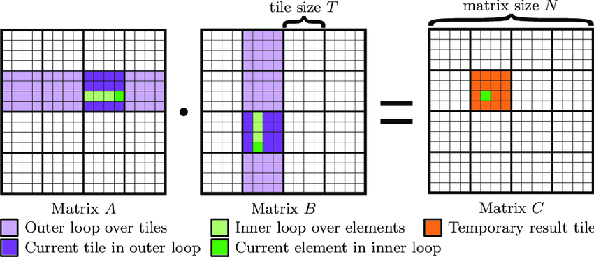 The Naive Approach:
- To calculate C(0)(0), fetch A(0)(0) and B(0)(0) from HBM, multiply, store result
- To calculate C(0)(1), fetch A(0)(0) again and B(1)(0) from HBM, multiply, store result
- Repeat for every element
Notice we fetched A(0)(0) twice. > For a 1000x1000 matrix, we’d fetch that same value 1000 times
The Tiled Approach:
- A group of threads cooperatively loads a 16x16 tile from A and a 16x16 tile from B into Shared Memory (the “Desk”)
- The threads perform every possible calculation using only the data currently on the Desk
- Only after exhausting all calculations with the current tiles do they return to HBM for the next tiles
By loading A(0)(0) once onto the Desk and using it to calculate 16 different output values, we’ve reduced memory traffic by 16x. This concept is formalized as Arithmetic Intensity:
Arithmetic Intensity = (FLOPs performed) / (Bytes moved)
- Low Intensity: Move 1 byte, do 1 operation. (Memory-bound)
- High Intensity: Move 1 byte, do 100 operations. (Compute-bound)
Good GPU kernels aim for high arithmetic intensity by maximizing data reuse. For more Info check Tiling Technique
Precision: BF16 Advantage:
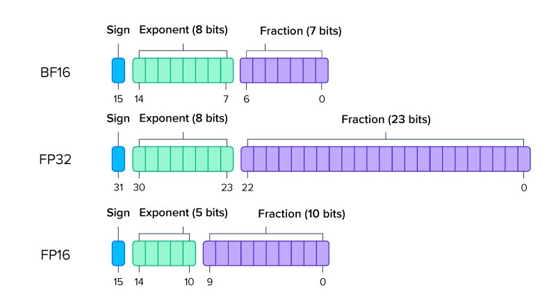 Standard machine learning uses FP32 (32-bit floating point). For a 175 billion parameter model like GPT-3:
175B parameters × 4 bytes/parameter = 700 GB
This doesn’t fit on a single GPU. Even if it did, moving 700 GB through memory at 3 TB/s takes ~230 milliseconds per pass(an eternity in GPU time). We shrink to 16 bits. But there are two formats:
FP16 (IEEE Half Precision):
- 1 sign bit
- 5 exponent bits
- 10 mantissa bits
- Range: ±65,504
- Precision: ~3 decimal digits
BF16 (Brain Float 16):
- 1 sign bit
- 8 exponent bits (same as FP32!)
- 7 mantissa bits
- Range: ±3.4×10³⁸ (same as FP32)
- Precision: ~2 decimal digits
The 8-bit exponent is critical. During backpropagation, gradients can explode (>65,504) or vanish (<10⁻⁵). FP16 hits overflow/underflow, producing NaNs that crash training → BF16’s extended range prevents this
Why this matters: You can simply cast FP32 activations to BF16, train, and cast back without elaborate loss scaling schemes. This is why every major lab (Google, Meta, OpenAI) defaults to BF16 for pre-training
- Memory saved: 700 GB → 350 GB
- Bandwidth saved: 2x faster data movement
- Training stability: No NaN crashes
Layer 2: Parallel GPU Training
A single H100 has 80 GB of memory. Modern LLMs are way big than that, the model doesn’t fit, even if it did, training on one GPU would take years and we need to distribute across hundreds or thousands of GPUs
Data Parallelism:
The model fits on one GPU, but if the dataset is enormous, we copy the entire model onto every GPU. Each GPU processes a different batch of data
Take a simple analogy of Chefs working together:
- 100 chefs (GPUs) all have the exact same recipe (model)
- Each chef gets different ingredients (data batch)
- Chef 1 tastes their pot: “Needs +5g salt”
- Chef 2 tastes their pot: “Needs -3g salt”
- Chef 3 tastes their pot: “Needs +2g salt”
If each chef just changed their own recipe independently, they’d drift apart. Instead, they have a conference call:
Average feedback = (+5 - 3 + 2) / 3 = +1.33g salt
Everyone adds exactly 1.33g of salt
In neural networks, this “feedback” is the gradient (∇W). The “conference call” is the AllReduce communication primitive
The Training Loop:
- Forward Pass: Each GPU computes predictions on its batch
- Backward Pass: Each GPU computes gradients ∇W_local
- AllReduce: Average all gradients across GPUs ∇W_global = (∇W_GPU1 + ∇W_GPU2 + … + ∇W_GPU100) / 100
- Optimizer Step: Every GPU updates weights identically
W_new = W_old - learning_rate × ∇W_global
After step 4, every GPU has the exact same weights again, ready for the next iteration
Pipeline Parallelism:
 #Q The model has 96 layers and cannot fit on one GPU, how can we train now ?
A We use Vertical slicing. Put layers 1-24 on GPU A, layers 25-48 on GPU B, layers 49-72 on GPU C, layers 73-96 on GPU
You can take a simple analogy of a Car Assembly:
- GPU 1 builds the chassis (first 24 layers)
- GPU 2 installs the engine (next 24 layers)
- GPU 3 adds the interior (next 24 layers)
- GPU 4 applies the paint (final 24 layers)
and the processing goes like
- Time Step 1: GPU 1 processes Batch 1 → GPU 2 idle → GPU 3 idle → GPU 4 idle
- Time Step 2: GPU 1 processes Batch 2 → GPU 2 processes Batch 1 → GPU 3 idle → GPU 4 idle
- Time Step 3: GPU 1 processes Batch 3 → GPU 2 processes Batch 2 → GPU 3 processes Batch 1 → GPU 4 idle
- Time Step 4: GPU 1 processes Batch 4 → GPU 2 processes Batch 3 → GPU 3 processes Batch 2 → GPU 4 processes Batch 1
Here, GPUs 2, 3, 4 aren’t doing anything for the first three time steps
To fix this we do Micro-Batching
 Instead of processing one large batch, we split it into many micro-batches and push them through the pipeline back-to-back:
μBatch 1 → GPU 1 → GPU 2 → GPU 3 → GPU 4
μBatch 2 → GPU 1 → GPU 2 → GPU 3
μBatch 3 → GPU 1 → GPU 2
μBatch 4 → GPU 1
After the initial ramp-up, all GPUs are busy simultaneously. Modern implementations (GPipe, PipeDream, Megatron-LM) use sophisticated schedules to minimize the bubble
The Gradient Synchronization Problem: In pipeline parallelism, different micro-batches are at different stages of the forward/backward pass. We accumulate gradients from all micro-batches before doing the AllReduce and weight update. This maintains consistency
Tensor Parallelism:
 #Q A single layer has a weight matrix so large (e.g., 12,288 × 12,288 in GPT-3) that even one layer doesn’t fit in one GPU’s memory, how can we train different matrix of same layers on different GPUs ?
A Horizontal slicing. Split the weight matrix itself across multiple GPUs
- The matrix is a 50-foot-long sofa
- Even with the cushions off (BF16, quantization), it’s too heavy to lift alone
- Solution: You lift the left half, your friend lifts the right half, and you move it together
 A Transformer block consists of an MLP (Multi-Layer Perceptron) and Attention. Let’s look at the MLP Y = B(A(X))
- Column Parallel Layer (A): We split matrix A vertically
- GPU 1 calculates Y_{1} = X × A_{1}
- GPU 2 calculates Y_{2} = X × A_{2}
- Result: Each GPU has a part of the output vector. No communication needed yet
- Row Parallel Layer (B): We split matrix B horizontally
- GPU 1 takes Y_{1} and calculates Z_{1} = Y_{1} × B_{1}
- GPU 2 takes Y_{2} and calculates Z_{2} = Y_{2} × B_{2}
- Critical Step: The true output Z is the sum of Z_{1} + Z_{2}
Each GPU starts with local gradients (1.0, 2.0, 3.0) GPUs share and reduce to compute average (2.0) Final average synchronized across all GPUs. Summing or aggregating the values from all devices. Redistributing the aggregated result (average in this case) back to all GPUs
- Forward Pass: requires an AllReduce at the end of the Row Parallel layer to sum the partial results (Z_{1} + Z_{2}) so the full Z can be passed to the residual connection and LayerNorm
- Backward Pass: The gradient flow mirrors this. We need an AllReduce to synchronize gradients before they flow back into the Column Parallel layer
The Communication Pattern:
- Forward pass: AllReduce (Sum)
- Backward pass: AllReduce (Sum)
This makes Tensor Parallelism extremely “chatty” - it needs to synchronize inside every single Transformer block
Combining All Three - Data Parallelism, Pipeline Parallelism and Tensor Parallelism: Let’s say we have
- Total GPUs: 512 (64 nodes × 8 GPUs/node)
- Model: 175B parameters
- Goal: Fit the model and maximize throughput
Configuration:
- Tensor Parallelism (TP): 8 (one node)
- Keeps TP communication on NVLink (900 GB/s)
- Pipeline Parallelism (PP): 8 (8 nodes stacked)
- Splits 96 layers into 8 stages of 12 layers each
- Now we have one “Model Replica” spanning 8 nodes (64 GPUs)
- Data Parallelism (DP): 8 (replicate the pipeline)
- 512 total GPUs / 64 GPUs per replica = 8 replicas
- Each replica processes different data
The Math: Total parameters: 175B Memory per parameter (BF16): 2 bytes Total model size: 350 GB
- Per GPU (with TP=8): 350 GB / 8 = 43.75 GB (fits in 80 GB H100)
- Effective batch size: 8 micro-batches × 8 pipeline stages × 8 data replicas = 512 samples per step
- Throughput: Each replica processes 8 micro-batches per pipeline flush 8 replicas × 8 micro-batches = 64 total batches processed in parallel
Layer 3: Infrastructure Layer(Cluster & Orchestration)
The Node and The Network:
A node is a single server box, typically containing 8 GPUs
In a data center, we might have:
1 Node = 8× H100 GPUs + 2× AMD EPYC CPUs + 2 TB RAM + 4× 400G InfiniBand NICs
These nodes are racked and cabled together to form a cluster
The Critical Constraint: Communication Speed
- Inside a Node (NVLink): Bandwidth: 900 GB/s between GPUs Latency: ~1 microsecond
- Between Nodes (InfiniBand): Bandwidth: 400 Gb/s = 50 GB/s Latency: ~5 microseconds
NVLink is roughly 18x faster than the inter-node network. This speed differential dictates how we map our parallelism strategies to hardware
The Mapping:
- Tensor Parallelism (TP)
- Requires AllReduce after every layer. Extremely chatty
- Constraint: Typically must stay within one node to use NVLink. (Exception: Newer clusters with GH200/NVL72 can span NVLink across racks, but standard H100 clusters are node-bound)
- Pipeline Parallelism (PP)
- Passes activations between stages. Moderate chattiness
- Tolerance: Can span nodes, but prefer fast inter-node connections
- Data Parallelism (DP)
- Only synchronizes once per optimizer step (after all micro-batches)
- Tolerance: Works fine across slow network
Fault Tolerance
MTBF (Mean Time Between Failures) of a single GPU: ~10 years MTBF of a cluster of 10,000 GPUs: ~10 years / 10,000 = ~9 hours
Q Why We Don’t Use Live Redundancy ?
A In databases, we might replicate data across nodes so if one dies, another takes over. In DL training, this is prohibitively expensive:
- Speed: Spreading TP across nodes for redundancy would kill performance (18x slower)
- Cost: Running 2x the GPUs to have a hot standby doubles your bill
The Checkpoint Strategy: Every N steps (e.g., every 100 steps = ~5 minutes), we save the model state to persistent storage (e.g., distributed filesystem):
checkpoint = {
	'model_state_dict': model.state_dict(),
	'optimizer_state_dict': optimizer.state_dict(),
	'step': current_step,
	'rng_state': torch.get_rng_state(),
}
torch.save(checkpoint, f'ckpt_step_{current_step}.pt')
On Failure:
- The training job crashes
- Orchestrator (Kubernetes/Slurm) detects crash
- Bad node is removed; replacement is allocated
- Job restarts from last checkpoint
- Lost progress: ~5 minutes of training
This is a fail-stop model, not fail-over. We don’t prevent the crash; we recover quickly
Bottlenecks
- The Activation Memory Problem: When we discuss model size, we often forget about activations - the intermediate tensors produced during the forward pass
- For a Transformer layer:
- Input: (batch, seq_len, hidden_dim)
- Attention: Stores Q, K, V matrices → 3 × batch × seq_len × hidden_dim
- Attention Scores: batch × num_heads × seq_len × seq_len (the memory killer)
- MLP: Stores intermediate → batch × seq_len × (4 × hidden_dim)
- For GPT-3 with:
- batch_size = 1024
- seq_len = 2048
- hidden_dim = 12,288
- num_layers = 96
- The self-attention score matrix alone: 1024 × 96 heads × 2048 × 2048 × 2 bytes (BF16) = 822 GB. This doesn’t fit in GPU memory! We need activation checkpointing (also called gradient checkpointing)
- The Trade-off:
- Normal training:
- Forward: Store all activations → Backward: Use stored activations
- Memory: High, Time: Fast
- Activation checkpointing:
- Forward: Store only some activations → Backward: Recompute others
- Memory: Low (1/N), Time: Slow (1.3x)
- We typically checkpoint every K layers (e.g., K=4). During backward pass, we recompute the activations for layers between checkpoints
- Normal training:
- Straggler Nodes
- AllReduce is synchronous - it’s only as fast as the slowest GPU
- GPU 0-98: Finished their computation in 10 seconds
- GPU 99: Still computing (thermal throttling, bad PCIe lane, noisy neighbor)
- Result: Everyone waits for GPU 99
- Detection: Monitor per-rank step times. If one rank is consistently 10% slower, investigate hardware
- Mitigation: Dynamic batch sizing, straggler replication (Facebook’s approach)
- Gradient Explosion/Vanishing
- Even with BF16, gradients can become problematic
- Gradient Clipping:
# Compute gradient norm across all GPUs grad_norm = torch.nn.utils.clip_grad_norm_(model.parameters(), max_norm=1.0) # This internally does an AllReduce of gradient norms! - If gradients exceed max_norm, they’re scaled down
- Reproducibility: The RNG Problem
- Each GPU has a random number generator (for dropout, data shuffling). for reproducible training:
def set_seed (rank, seed): torch.manual_seed(seed + rank) # Each rank gets different seed np.random.seed(seed + rank) random.seed(seed + rank) - But even with seeds set, NCCL AllReduce order can change results slightly due to floating-point non-associativity: (a + b) + c ≠ a + (b + c) (in floating point)
- True reproducibility requires deterministic CUDA kernels:
torch.use_deterministic_algorithms (True) - But this disables many optimized kernels, slowing training by 20-50%
- Each GPU has a random number generator (for dropout, data shuffling). for reproducible training:
Optimizations
- Gradient Accumulation: Simulating Larger Batches
- Your GPU can fit batch=16, but you want effective batch=128 for better convergence
accumulation_steps = 8 # 16 * 8 = 128 optimizer.zero_grad() for i, batch in enumerate (dataloader): loss = model(batch) / accumulation_steps # Scale loss loss.backward() if (i + 1) % accumulation_steps 0: optimizer.step() optimizer.zero_grad() - Trade-off:
- Memory: Gradients accumulate across micro-batches (no extra cost)
- Time: Updates happen 8× less frequently (slower convergence per step)
- Math: Identical to true batch=128
- Mixed Precision: BF16 Compute, FP32 Accumulation Even with BF16, we keep a master copy of weights in FP32:
model_bf16 model.bfloat16() # Weights in BF16 optimizer = Adam (model.parameters()) # Stores FP32 master weights internally with torch.cuda.amp.autocast(dtype=torch.bfloat16): loss = model_bf16(input) # Compute in BF16 loss.backward() # Gradients in BF16 optimizer.step() # Updates FP32 master, then copies to BF16 - Why:
- BF16 math is 2× faster (fewer bits to move)
- FP32 accumulation prevents rounding errors from compounding
- Negligible memory overhead (optimizer already stores FP32)
- Your GPU can fit batch=16, but you want effective batch=128 for better convergence
- Fused Kernels: Reducing Memory Round-Trips
x = layer_norm(x) # 3 separate kernels, 3 memory round-trips x = gelu(x) x = dropout(x, p=0.1)- Fused Version
# 1 kernel, 1 memory round-trip x = fused_layer_norm_gelu_dropout(x, p=0.1) # Libraries like Apex and xFormers provide fused operations: from xformers.ops import memory_efficient_attention # Fused attention (FlashAttention) out = memory_efficient_attention(Q, K, V) - Speedup: 10-20% for attention-heavy models (Transformers)
- Fused Version
- Overlap Communication and Computation
- In standard Data Parallelism, we do:
- Compute gradients (10 seconds)
- AllReduce gradients (7 seconds) ← GPUs idle during this
- Optimizer step (1 second)
- With overlapping:
- Start computing gradients for layer 96
- As soon as layer 96 gradients are ready, launch AllReduce for them
- While AllReduce is happening, compute gradients for layer 95
- When layer 95 is ready, launch its AllReduce
- By the time forward/backward finishes, most AllReduce is already done
model = DistributedDataParallel( model, bucket_cap_mb=25, # AllReduce groups of 25MB at a time gradient_as_bucket_view=True # Avoid memory copy ) - Speedup: Can hide 50-80% of communication time
- In standard Data Parallelism, we do:
Note:
AllReduce
 The Problem:
- We have N GPUs
- Each GPU has a vector of gradients (e.g., 1 GB)
- We need every GPU to end up with the sum of all vectors
Naive Approach:
- GPU 0 collects all vectors (requires N sends to GPU 0)
- GPU 0 sums them (only one GPU working)
- GPU 0 broadcasts result to everyone (requires N sends from GPU 0)
Total data movement: 2N × vector_size
Problem: GPU 0 is a bottleneck
Ring AllReduce:
Arrange GPUs in a logical ring. Each GPU talks only to its neighbors
GPU 0 <> GPU 1 <> GPU 2 <> GPU 3 <> GPU 0 (wraps around)
- Phase 1: Reduce-Scatter
- Split each vector into N chunks. In N-1 steps, each GPU sends one chunk to its neighbor and receives one from the other neighbor. Each GPU accumulates the received chunks
- After N-1 steps: Each GPU holds the sum of one chunk from all GPUs
- Phase 2: AllGather
- In another N-1 steps, each GPU sends its summed chunk around the ring so everyone gets all chunks. After N-1 more steps: Every GPU has the complete summed vector
- Total data movement: 2 × (N-1) / N × vector_size ≈ 2 × vector_size
- Independent of N! Whether we have 8 GPUs or 8,000 GPUs, each GPU sends/receives roughly 2× the vector size
- NCCL (NVIDIA Collective Communications Library) implements optimized versions of Ring AllReduce and other algorithms, automatically choosing the best one based on message size and topology
FlashAttention
 The attention mechanism is a perfect example of a memory-bound operation that can be fixed with Tiling
Standard Attention:
Q, K, V = Linear(X) # [batch, seq, dim]
Scores = Q @ K.T # [batch, seq, seq] <- HUGE!
Probs = softmax (Scores) # Still [batch, seq, seq]
Out = Probs @ V # [batch, seq, dim]
The problem: Scores is quadratic in sequence length. For seq=2048, this is 4M elements per batch item. We write it to HBM, read it back for softmax, write again, read again for the multiplication with V
FlashAttention (Dao et al., 2022) applies tiling:
- Split Q, K, V into blocks
- Load one block into SRAM
- Compute attention for that block without writing to HBM
- Accumulate partial outputs
- Move to next block
 The Result:
- Memory I/O: O(seq²) → O(seq²/M) (Sub-quadratic / Near-linear)
- Speed: 2-4x faster
- Exact result: Mathematically equivalent to standard attention
Zero Redundancy Optimizer (ZeRO)
 In standard Data Parallelism, each GPU stores:
- Model parameters (W)
- Gradients (∇W)
- Optimizer states (momentum, variance for Adam)
For Adam optimizer:
- Memory per GPU = 2 bytes (W) + 2 bytes (∇W) + 8 bytes (optimizer states) = 12 bytes per parameter
For a 175B parameter model: 175B × 12 = 2.1 TB per GPU
- ZeRO Stage 1: Shard optimizer states across GPUs. Each GPU stores: Full W, Full ∇W, 1/N of optimizer states Memory: 4 + 8/N bytes per parameter
- ZeRO Stage 2: Shard gradients too. Each GPU stores: Full W, 1/N of ∇W, 1/N of optimizer states Memory: 2 + 2/N + 8/N bytes per parameter
- ZeRO Stage 3: Shard everything, including the model. Each GPU stores: 1/N of W, 1/N of ∇W, 1/N of optimizer states Memory: 12/N bytes per parameter
The Trade-off: Each stage adds more communication. ZeRO-3 requires AllGather before every forward/backward to reconstruct the full parameters. But it allows training models 8-64x larger than standard DP