Linear Regression

At its core, linear regression is about finding a line that best summarizes the relationship between our input (x) and output (y). Imagine our data as points on a graph. Our goal is to draw one straight line through those points that is as close to all of them as possible

For Example, Let’s use our student data

Hours Studied (x)	Exam Score (y)
1	2
2	4
3	5
4	4
5	5
If we plot this, we get a scatter of points

Exam Score
6 |                          
5 |            ●        ●
4 |        ●        ●
3 |
2 |    ●
1 |
0 +--------------------------------
    0   1   2   3   4   5   6
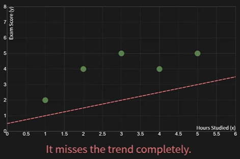
          Hours Studied

Now, let’s try to draw two different lines through this data to see what “fitting” means.

1. Bad fit
2. Good fit

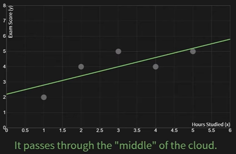
Visually, the green line is a better fit. Our model is the equation for that line
The Line Equation:
The formula for any straight line is: $\hat{y}=w\cdot x+b$

• $\hat{y}$ (y-hat): This is our predicted output value (e.g., predicted exam score).
• $x$: This is our input value (e.g., hours studied).
• $w$: The weight (or slope). It controls the steepness of the line. A bigger w means that for every hour studied, the predicted score increases more.
• $b$: The bias (or y-intercept). It’s the value of $\hat{y}$ when $x=0$. You can think of it as a baseline prediction.

Finding the “best fit line” is just a search for the optimal values of w and b But this is for one input, and when we’re expanding to More Inputs

Q What if we want to predict a house price based on its size (x1) and the number of bedrooms (x2)? The model scales easily. Instead of a line, we are now fitting a plane ?
A $\hat{y}=w_1\cdot x_1+w_2\cdot x_2+b$ The principle is identical: find the weights (w1, w2) and bias (b) that make the predictions closest to the actual house prices

Loss Function

Our eyes can tell us the green line is better than the red one. But to find the best line, a computer needs a precise, mathematical way to measure how “bad” any given line is. This measurement is called the loss function. A high loss means a bad fit. A low loss means a good fit
Our goal is to find the w and b that give the lowest possible loss

Mean Squared Error (MSE):
The most common loss function for regression is the Mean Squared Error. We calculate it in three steps for every point in our data: $J(w,b)=\frac{1}{n}{\sum }_{i=1}^n({\hat{y}}_i-y_i{)}^2$

1. Calculate the error: For a single point, find the difference between the predicted value and the actual value. This vertical distance is called the residual error = predicted_y - actual_y or ${\hat{y}}_i-y_i$
2. Square the error: We square the error to get rid of negative signs (so errors don’t cancel each other out) and to penalize large errors much more than small ones. An error of 3 becomes 9, while an error of 10 becomes 100 squared_error = (error)^2
3. Take the mean: We calculate the squared error for all our data points and then take the average. This gives us a single number that represents the overall quality of our line

Calculating Loss for Two Lines:
Let’s prove with math that our visual intuition was right

• Data: xs = [1, 2, 3, 4, 5], ys = [2, 4, 5, 4, 5]
• Line 1 (Bad Guess): $\hat{y}=1\cdot x+1$ (Here, w=1, b=1)
• Line 2 (Better Guess): $\hat{y}=0.6\cdot x+2.5$ (Here, w=0.6, b=2.5)

Calculation for Line 1 (w=1, b=1):

x	y (actual)	$\hat{y}=1x+1$ (predicted)	Error ($\hat{y}-y$)	Squared Error
1	2	2	0	0
2	4	3	-1	1
3	5	4	-1	1
4	4	5	1	1
5	5	6	1	1
			Sum:	4
MSE for Line 1 = (Sum of Squared Errors) / n = 4 / 5 = 0.8
Calculation for Line 2 (w=0.6, b=2.5):

x	y (actual)	$\hat{y}=0.6x+2.5$ (predicted)	Error ($\hat{y}-y$)	Squared Error
1	2	3.1	1.1	1.21
2	4	3.7	-0.3	0.09
3	5	4.3	-0.7	0.49
4	4	4.9	0.9	0.81
5	5	5.5	0.5	0.25
			Sum:	2.85
MSE for Line 2 = (Sum of Squared Errors) / n = 2.85 / 5 = 0.57
Result: Line 2 has a lower MSE (0.57) than Line 1 (0.8). The math confirms it is a better fit

Gradient Decent

We now have a model (y = w*x + b) and a way to score it (MSE). The final piece is the process for finding the specific w and b that result in the lowest possible MSE score. This process is called training, and the most common algorithm for it is Gradient Descent

Intuition: Walking Down a Mountain in the Fog

• Imagine the loss function as a giant, hilly landscape. Every possible combination of w and b is a location on this landscape, and the altitude at that location is the MSE score. Our goal is to find the bottom of the lowest valley (the minimum MSE)
• The problem is, we’re in a thick fog. We can’t see the whole landscape. All we can do is feel the slope of the ground right where we’re standing

Gradient Descent is a simple strategy:

1. Check the slope: Feel which direction is steepest downhill. In math, this slope is called the gradient
2. Take a small step: Take one step in that downhill direction
3. Repeat: From your new position, repeat the process

By taking many small steps, you will eventually walk down the hill and settle at the bottom of the valley

Algorithm: This “walking” process translates into a simple update rule for our parameters, w and b:

• Update Rule for w: w_new = w_old - learning_rate * gradient_w
• Update Rule for b: b_new = b_old - learning_rate * gradient_b

Two new terms here:

• learning_rate ($\alpha$): This controls the size of our downhill step. If it’s too big, we might overshoot the valley. If it’s too small, it could take forever to get to the bottom. It’s a hyperparameter you choose
• gradient_w and gradient_b: These are the calculated slopes for w and b. They tell us how a small change in w or b will affect the MSE. The formulas for these gradients, derived from the MSE function, are:
  • $gradien{t}_w=\frac{\partial J}{\partial w}=\frac{2}{n}{\sum }_{i=1}^n({\hat{y}}_i-y_i)\cdot x_i$
  • $gradien{t}_b=\frac{\partial J}{\partial b}=\frac{2}{n}{\sum }_{i=1}^n({\hat{y}}_i-y_i)$

For example, let us understand: One Step of Gradient Descent
Performing a single training step

• Data: xs = [1, 2, 3, 4, 5], ys = [2, 4, 5, 4, 5]
• Hyperparameter: Let’s choose a learning_rate of 0.01
• Step 0: Initialize. We start with a random guess. Let’s begin at w = 0.0 and b = 0.0. This is our “before” state

The MSE for this initial line ($\hat{y}=0$) is high: $MS{E}_{before}=\frac{(0-2{)}^2+(0-4{)}^2+(0-5{)}^2+(0-4{)}^2+(0-5{)}^2}{5}=\frac{4+16+25+16+25}{5}=17.2$

• Step 1: Calculate the Gradients. We use our formulas and data to find the slope at our current position (w=0, b=0)

x	y	$\hat{y}=0x+0$	Error ($\hat{y}-y$)	Error * x
1	2	0	-2	-2
2	4	0	-4	-8
3	5	0	-5	-15
4	4	0	-4	-16
5	5	0	-5	-25
			Sum = -20	Sum = -66
Now, plug the sums into the gradient formulas (n=5):

• gradient_w = (2 / 5) * (-66) = -26.4
• gradient_b = (2 / 5) * (-20) = -8.0

These gradients tell us the direction of steepest ascent. To go downhill, we move in the opposite direction

• Step 2: Update the Parameters. We use our update rule to take one small step

  • w_new = w_old - learning_rate * gradient_w

  • w_new = 0.0 - 0.01 * (-26.4) = 0.264

  • b_new = b_old - learning_rate * gradient_b

  • b_new = 0.0 - 0.01 * (-8.0) = 0.08

Result:

• Before (Step 0): w = 0.0, b = 0.0, MSE = 17.2
• After (Step 1): w = 0.264, b = 0.08, MSE = 11.45 (calculated by plugging the new w and b into the MSE formula)

The process simply repeats this exact calculation many times (epochs), with w and b getting closer to the optimal values with every step

Convergence Over Multiple Steps:
If we continue the process with a learning rate of 0.05, the table below shows how w and b gradually converge to the optimal values (w = 0.6, b = 2.2):

Step	w	b	MSE
0	0.0000	0.0000	17.2000
1	1.3200	0.4000	1.6464
2	1.0680	0.3640	1.1047
5	1.0807	0.4655	1.0276
10	1.0412	0.6072	0.9418
20	0.9720	0.8569	0.8084
50	0.8231	1.3946	0.5981
100	0.6951	1.8566	0.5015
200	0.6173	2.1376	0.4807
500	0.6001	2.1996	0.4800
1000	0.6000	2.2000	0.4800
Optimal	0.6000	2.2000	0.4800
By step 1000, we’ve essentially converged to the optimal solution that the Normal Equation gives us instantly

Normal Equation

Instead of taking thousands of small steps with Gradient Descent, we can use a direct formula to solve for the optimal w and b in one single calculation. This is called the Normal Equation
It’s the mathematical equivalent of seeing the entire loss landscape from above and simply pointing to the lowest point, rather than feeling your way down in the fog

The intuition comes from basic calculus: the minimum of a function is where its slope (derivative) is zero. The Normal Equation is what you get when you:

1. Write the MSE loss function using matrix notation
2. Take the derivative with respect to your parameters (w and b)
3. Set that derivative to zero
4. Solve for the parameters

The resulting formula is: $\theta =(X^{T}X{)}^{-1}{X}^{T}y$

• $\theta$ (theta): A vector containing all our model parameters. In our case, $\theta =\left[\begin{array}{c}b\\ w\end{array}\right]$
• $X$: The design matrix, which is our input data xs with an extra column of ones added for the bias term
• $y$: The vector of our actual output values

Applying the Normal Equation to an Example:
Let’s solve for the optimal w and b for our student data in one go

• Data: xs = [1, 2, 3, 4, 5], ys = [2, 4, 5, 4, 5]

Step 1: Construct the matrix X and vector y We need to add a column of ones to our xs to account for the bias term b

$$X=\left[\begin{array}{cc}1& 1\\ 1& 2\\ 1& 3\\ 1& 4\\ 1& 5\end{array}\right],y=\left[\begin{array}{c}2\\ 4\\ 5\\ 4\\ 5\end{array}\right]$$

Step 2: Calculate $X^{T}X$

$$X^T=\left[\begin{array}{ccccc}1& 1& 1& 1& 1\\ 1& 2& 3& 4& 5\end{array}\right]$$ $$X^{T}X=\left[\begin{array}{ccccc}1& 1& 1& 1& 1\\ 1& 2& 3& 4& 5\end{array}\right]\left[\begin{array}{cc}1& 1\\ 1& 2\\ 1& 3\\ 1& 4\\ 1& 5\end{array}\right]=\left[\begin{array}{cc}5& 15\\ 15& 55\end{array}\right]$$

Step 3: Calculate the inverse, $(X^{T}X{)}^{-1}$ For a 2x2 matrix $\left[\begin{array}{cc}a& b\\ c& d\end{array}\right]$, the inverse is $\frac{1}{ad-bc}\left[\begin{array}{cc}d& -b\\ -c& a\end{array}\right]$ Determinant ($ad-bc$) = (5 * 55) - (15 * 15) = 275 - 225 = 50

$$\left[\begin{array}{cc}55& -15\\ -15& 5\end{array}\right]=\left[\begin{array}{cc}1.1& -0.3\\ -0.3& 0.1\end{array}\right]$$

Step 4: Calculate $X^{T}y$

$$X^{T}y=\left[\begin{array}{ccccc}1& 1& 1& 1& 1\\ 1& 2& 3& 4& 5\end{array}\right]\left[\begin{array}{c}2\\ 4\\ 5\\ 4\\ 5\end{array}\right]=\left[\begin{array}{c}2+4+5+4+5\\ 2+8+15+16+25\end{array}\right]=\left[\begin{array}{c}20\\ 66\end{array}\right]$$

Step 5: Calculate the final result, $\theta =(X^{T}X{)}^{-1}{X}^{T}y$

$$\theta =\left[\begin{array}{cc}1.1& -0.3\\ -0.3& 0.1\end{array}\right]\left[\begin{array}{c}20\\ 66\end{array}\right]=\left[\begin{array}{c}(1.1\ast 20)+(-0.3\ast 66)\\ (-0.3\ast 20)+(0.1\ast 66)\end{array}\right]=\left[\begin{array}{c}22-19.8\\ -6+6.6\end{array}\right]=\left[\begin{array}{c}2.2\\ 0.6\end{array}\right]$$

The Normal Equation gives us the exact optimal parameters in one calculation:

• $b=2.2$
• $w=0.6$

The best fit line for our data is $\hat{y}=0.6\cdot x+2.2$. This is the mathematical bottom of the loss valley that Gradient Descent was slowly stepping towards

Limitations:

Feature	Gradient Descent	Normal Equation
Process	Iterative, takes many small steps.	Direct, one-shot calculation.
Scalability	Works well with huge datasets (millions of features).	Computationally expensive for many features (inverting a large matrix is slow).
Learning Rate	Requires choosing a learning rate, $\alpha$.	No hyperparameters to tune.
When to Use	The default for most large-scale ML problems.	Excellent for smaller datasets where the number of features is not too large (e.g., < 10,000).