Quantization

Quantization means approximating the decimal places in the model weights(decreasing the floating point places). The goal is to represent a wide range of continuous floating-point numbers using a small, finite set of integers. This entire process is a simple mapping governed by two parameters: a scale factor and a zero-point
Q How a Float is Stored (FP32) ?
A Computers represent decimal numbers using a standard format called IEEE 754 single-precision floating-point, or FP32. Every FP32 number consumes 32 bits, divided into three parts:

Component	Bits	Purpose
Sign (S)	1 bit	0 for positive, 1 for negative.
Exponent (E)	8 bits	Determines the number’s magnitude (range).
Mantissa (M)	23 bits	Stores the actual digits of the number (precision).
The value is reconstructed using the formula: Value = (-1)^S * (1 + Mantissa) * 2^(Exponent - 127). For example, here is the representation for the number 3.5

1. Sign (S): The number is positive, so S = 0
2. Binary Form: 3.5 in binary is 11.1
3. Scientific Notation: Normalize this to 1.11 x 2^1
4. Exponent (E): The power is 1. We add the bias 127: E = 1 + 127 = 128. In 8-bit binary, this is 10000000
5. Mantissa (M): The fractional part from the scientific notation is .11. We pad this to 23 bits: 11000000000000000000000

Putting it all together, 3.5 in FP32 is: [0] [10000000] [11000000000000000000000] (1 bit) (8 bits) (23 bits)

The Problem: FP32 is Too Big
This representation is precise but inefficient for inference

• Memory Cost: Each parameter takes 32 bits, or 4 bytes. For a 7-billion parameter model: 7,000,000,000 parameters * 4 bytes/parameter = 28,000,000,000 bytes = 28 GB of VRAM
• Bandwidth Cost: The GPU is starved waiting for these 28 GB of weights to be moved from VRAM to the compute cores. This memory transfer is often the true bottleneck

The Solution: Mapping to a Simpler Format (INT8) Imagine you have a small tensor of weights that fall within the range [-3.5, 3.5]
weights_fp32 = (1.2, -3.5, 0.8, 2.1, -1.9, 3.5)
Our task is to represent these numbers using INT8, which can only hold values between [-128, 127]
Q How do we map every possible number from -3.5 to 3.5 onto one of the 256 available integer “buckets”? #A

1. Calculate the Scale (S): The scale is our “step size.” It tells us how many float units correspond to a single integer unit.

   • The total span of our float values is 3.5 - (-3.5) = 7.0
   • The total span of our INT8 values is 127 - (-128) = 255
   • Scale (S) = Float Range / Integer Range = 7.0 / 255 ≈ 0.02745

   This means for every step we take in the integer world (e.g., from 10 to 11), we are moving approximately 0.02745 in the float world

2. Calculate the Zero-Point (Z): The zero-point is an offset or “shift.” It ensures that the floating-point value 0.0 maps correctly to an integer. Since our float range [-3.5, 3.5] is perfectly symmetric around zero, we can align its zero with the integer zero

   • Zero-Point (Z) = 0
   • This special case is called Symmetric Quantization and is standard for model weights

The Formal Algorithm (Affine Quantization)

1. Quantization (Float → Int): $q=\text{clamp}\left(\text{round}\left(\frac{x}{S}+Z\right),q_{min},q_{max}\right)$
   • x: The original float value (e.g., 1.2)
   • S: The scale factor we calculated
   • Z: The zero-point we calculated
   • round(): Standard rounding to the nearest integer
   • clamp(): Ensures the result stays within the valid integer range ([-128, 127])
2. Dequantization (Int → Float):  $\hat{x}=S(q-Z)$
   • q: The quantized integer value
   • x̂: The reconstructed (approximate) float value

For example, Let’s quantize our float x = 1.2 using S = 0.02745 and Z = 0

1. Scale: 1.2 / 0.02745 ≈ 43.71
2. Shift: 43.71 + 0 = 43.71
3. Round: round(43.71) = 44
4. Clamp: 44 is within [-128, 127], so no clamping is needed

So, the float 1.2 is represented by the integer 44
The error by dequantizing it back is x̂ = 0.02745 * (44 - 0) ≈ 1.2078. The error is very small!

Symmetric Quantization

This is the most common type for weights. The zero-point is fixed at 0

import numpy as np
 
def symmetric_quantize_int8(fp32_tensor):
    # For INT8, the max integer value is 127
    q_max = 127.0
 
    # 1. Find the absolute maximum float value to define the range
    abs_max = np.max(np.abs(fp32_tensor))
 
    # 2. Calculate the scale factor
    scale = abs_max / q_max
 
    # 3. Apply the quantization formula (Z=0)
    quantized_tensor = np.round(fp32_tensor / scale)
    quantized_tensor = np.clip(quantized_tensor, -128, 127).astype(np.int8)
 
    return quantized_tensor, scale
 
# --- Input ---
weights_fp32 = np.array([1.2, -3.5, 0.8, 2.1, -1.9, 3.5], dtype=np.float32)
 
# --- Output ---
quantized_weights, scale = symmetric_quantize_int8(weights_fp32)
print(f"Original FP32: {weights_fp32}")
print(f"Scale (S): {scale:.4f}")
print(f"Quantized INT8: {quantized_weights}")
dequantized_weights = quantized_weights.astype(np.float32) * scale
print(f"Dequantized FP32: {np.round(dequantized_weights, 4)}")

Mapping Table: Here is how our original weights map to the INT8 format

Original Float (x)	Calculation (x / S)	Rounded Int (q)	Dequantized Float (x̂)	Error (x - x̂)
1.2	1.2 / 0.0275 = 43.56	44	1.21	-0.01
-3.5	-3.5 / 0.0275 = -127.0	-127	-3.49	-0.01
0.8	0.8 / 0.0275 = 29.03	29	0.80	0.00
2.1	2.1 / 0.0275 = 76.22	76	2.09	+0.01
-1.9	-1.9 / 0.0275 = -68.96	-69	-1.90	0.00
3.5	3.5 / 0.0275 = 127.0	127	3.49	+0.01
The core idea: Find a scale factor to stretch or shrink the float range to fit the integer range. The error introduced is called quantization error

Weights-Only Quantization & Mixed Precision

Q Where do we apply it inside a real neural network?
A A neural network layer primarily does one simple thing: it performs a matrix multiplication Output = MatMul(Input_Data, Weights)
The key is to understand what these two components are

• Weights: Think of these as the model’s brain or its long-term memory. They contain all the knowledge learned during weeks of training. They are static, enormous, and are loaded into the GPU’s memory (VRAM) once. For a 7B model, this “brain” is the 28 GB of data we need to shrink
• Input Data (Activations): This is the stream of thought or the data that is actively flowing through the model right now. When we type a prompt, our words are turned into numbers that become the Input_Data for the first layer. The output of that layer then becomes the input for the next. These numbers are dynamic and change with every new request

Q What Do We Compress, Weights or the Input Data(Activations) or both ?
A Given the nature of these two components, the engineering choice becomes clear

1. Why We MUST Quantize Weights:
   • They are the memory problem. The weights are the massive, multi-gigabyte files that live permanently in VRAM. Compressing them from FP32 (or FP16) to INT8 gives us a 4x (or 2x) reduction in memory footprint, which is our primary goal
   • They are static. Since they don’t change during inference, we can quantize them once and store them in their compressed form
2. Why We Generally DON’T Quantize Activations:
   • They are transient. Activations are “in-flight” data. They are generated, used in one calculation, and then discarded. They don’t live in VRAM for long
   • They are computationally expensive to quantize. Compressing them would mean adding a quantize() step at the input of every layer and a dequantize() step at the output, adding overhead to the critical path for a minimal memory gain

This leads to the industry-standard approach: Weights-Only Quantization. We compress the large, static “brain” (weights) but keep the fast-moving “thoughts” (activations) in their high-precision format (usually FP16). This is also called a Mixed-Precision Approach

The On-the-Fly Dequantization:
Q How can you multiply an FP16 activation with an INT8 weight?
A We Don’t. Modern GPUs have specialized hardware to perform a clever, last-second conversion. Here is the step-by-step process for Y = MatMul(Activations, Weights):

1. Storage: The Weights tensor is stored in VRAM as INT8. Its corresponding Scale factor is stored nearby as an FP16 number. The Activations tensor arrives at the layer as a standard FP16 tensor
2. Load: The GPU’s compute core pulls the necessary INT8 weights and their scale from VRAM into its own extremely fast on-chip memory
3. Dequantize On-the-Fly: Inside the core, just nanoseconds before the multiplication, a specialized circuit dequantizes the weights back to FP16

$${\text{Temporary\_Weight}}_{FP16}=S\times {\text{Weight}}_{INT8}$$

4. Compute: The matrix multiplication is now performed with both inputs in the same high-precision format

$${\text{Y}}_{FP16}=\text{MatMul}({\text{Activations}}_{FP16},{\text{Temporary\_Weight}}_{FP16})$$

5. Discard: The Temporary_Weight is immediately discarded. It only existed for a fraction of a second in the core’s cache. The permanent Weight tensor in VRAM remains in its compressed INT8 form

This hardware-fused process gives us the best of both worlds: a 4x reduction in memory footprint from INT8 storage, and the full numerical accuracy of FP16 for the actual computation

Flow chart, illustrating the mixed-precision matrix multiplication process

------------------------------------------------------------------------
| Box 1: VRAM (Slow, Large Memory)                                     |
|   - [Tensor] Activations (FP16) - Size: Large, but transient         |
|   - [Tensor] Weights (INT8) - Size: Huge, compressed                 |
|   - [Vector] Scale Factors (FP16) - Size: Tiny                       |
------------------------------------------------------------------------
      |
      | Memory Bus (The Bottleneck We Are Solving)
      | Data Transferred: Activations (FP16) + Weights (INT8)
      |
      V
-------------------------------------------------------------------------
| Box 2: GPU Core (Fast, Small On-Chip Cache)                           |
|   1. [Operation] On-the-fly Dequantization                            |
|      Input: Weights (INT8), Scale (FP16)                              |
|      Output: Dequantized Weights (FP16) -> This is temporary!         |
|   2. [Operation] Matrix Multiplication                                |
|      Input A: Activations (FP16)                                      |
|      Input B: Dequantized Weights (FP16)                              |
|      Output: Result (FP16)                                            |
-------------------------------------------------------------------------

This hardware-fused process gives us the best of both worlds: a 4x reduction in memory footprint from INT8 storage, and the full numerical accuracy of FP16 for the actual computation. We have successfully reduced the memory required for our weights without significantly affecting the mathematical outcome

Handling Outliers:
The symmetric quantization method we’ve used so far, assumes that weight values are evenly distributed, but in reality, neural networks often contain a few “specialist” weights with extremely large magnitudes
For example, when we consider this tensor, which have a single massive outlier value
weights_fp32 = (1.2, -3.5, 0.8, 2.1, -1.9, 1000.0)

Now, when we quantize it using the same method as before

1. Find the Absolute Maximum: The abs_max is now 1000.0
2. Calculate the Scale (S): S = abs_max / q_max = 1000.0 / 127 ≈ 7.87
3. Apply Quantization q = round(x / S):
   • For x = 1.2: round(1.2 / 7.87) = round(0.15) = 0
   • For x = -3.5: round(-3.5 / 7.87) = round(-0.44) = 0
   • For x = 0.8: round(0.8 / 7.87) = round(0.10) = 0

The single outlier 1000.0 has inflated the scale factor so much that all the other smaller, important values are “squashed” into the integer 0. We have effectively erased their information

The problem is not the quantization algorithm itself, but the scope over which we apply it. Using one scale factor for an entire tensor is too coarse. The solution is to use multiple scale factors for smaller chunks of the tensor. This concept is called granularity
There are three common levels of granularity

1. Per-Tensor Quantization (The Flawed Baseline) This is what we have been doing. We calculate a single scale factor for the entire weight matrix
   • Pros: Simplest method, minimal overhead (only one scale factor to store)
   • Cons: Extremely sensitive to outliers, often leading to significant quality loss
2. Per-Channel Quantization (The INT8 Standard): Instead of one scale for the whole matrix, we calculate a separate scale factor for each row. In a linear layer, each row of the weight matrix corresponds to the connections for a single output neuron or “channel.” This is the most common method for INT8 quantization
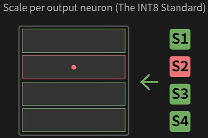
   • Pros: Effectively isolates outliers. An outlier in one row only affects the precision of that single row, leaving all other rows untouched
   • Cons: Requires storing more metadata (one scale factor per row instead of one for the whole matrix)

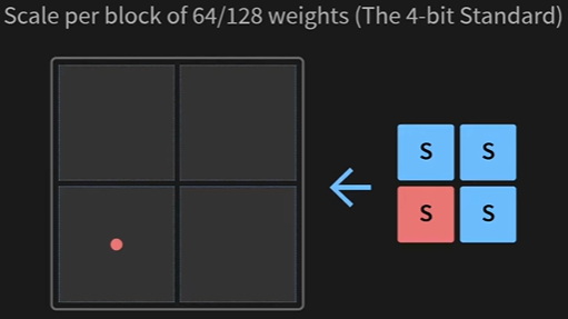
   # --- Code Snippet: Per-Channel Scale Calculation ---
   import numpy as np
    
   # A weight matrix with 3 rows (channels) and 4 columns
   weights_fp32 = np.array([
       [1.2, -0.5, 2.8, 0.9],   # Channel 1: max(abs) is 2.8
       [-1.5, 1000.0, 0.3, -2.1], # Channel 2: has a huge outlier
       [3.1, -2.2, -1.8, 1.1]    # Channel 3: max(abs) is 3.1
   ], dtype=np.float32)
    
   # Calculate scales per-row (axis=1 means operate along columns for each row)
   abs_max_per_channel = np.max(np.abs(weights_fp32), axis=1)
   scales_per_channel = abs_max_per_channel / 127.0
    
   print(f"Per-Channel Scales (S): {scales_per_channel}")
   # Output: [0.022, 7.87, 0.024]
   # Notice how the scale for Channel 2 is huge, but the others remain small and precise.

3. Group-wise Quantization (The 4-bit Standard): When we move to extremely low bit-widths like 4-bit, even per-channel quantization can lose too much information. The solution is to increase granularity even further. We take each row and divide it into smaller chunks called groups or blocks (e.g., of size 32, 64, or 128). Each group gets its own scale factor
   • Pros: The highest precision, as outliers are isolated to very small blocks of weights
   • Cons: The most metadata overhead. For a group size of 128, we store one scale factor for every 128 weights

Granularity	Best For	Quality	Overhead
Per-Tensor	Simple cases, no outliers	Lowest	Lowest
Per-Channel	INT8 Quantization	Good	Medium
Group-wise	4-bit Quantization	Highest	Highest
By calculating scale factors over smaller and smaller groups of numbers, we drastically reduce quantization error and preserve the performance of the model. This principle is what makes 4-bit quantization feasible

4-Bit Quantization

We’ve successfully compressed weights to INT8. To run even larger models on consumer hardware, we must push compression to the limit: 4-bit quantization. This halves the memory footprint again but requires us to be even more careful about precision and data storage

The Real-World Impact: VRAM Calculation
Let’s see what this means for a 7-billion parameter model. Remember, 1 byte = 8 bits

Format	Bits per Weight	Bytes per Weight	VRAM for 7B Model	Memory Savings (vs FP16)
FP16	16	2	14 GB	-
INT8	8	1	7 GB	2x
INT4	4	0.5	3.5 GB	4x
The Hardware Constraint: Packing Two Numbers in One Byte
A computer’s memory is addressed in chunks of bytes (8 bits). It’s impossible to read or write just 4 bits. To solve this, we must pack two 4-bit numbers into a single 8-bit byte

• The first 4-bit number occupies the lower half of the byte.
• The second 4-bit number is shifted to occupy the upper half.

Packing two 4-bit values (5 and 10) into one 8-bit byte

• A rectangle represents an 8-bit byte: (b7 | b6 | b5 | b4 | b3 | b2 | b1 | b0 )
• Value 5 (binary 0101) goes into the right half: (? | ? | ? | ? | 0 | 1 | 0 | 1)
• Value 10 (binary 1010) goes into the left half: (1 | 0 | 1 | 0 | 0 | 1 | 0 | 1)

The result is a single byte containing the packed information

The Algorithm: Smaller Range, Higher Granularity
The quantization math is the same, but our target integer range is now tiny: [-8, 7] (16 possible values). S = max(|x|) / 7 Because the range is so small, using a single scale for a large group of weights would destroy all precision. This is why group-wise quantization (calculating a scale for every 32, 64, or 128 weights) is essential for 4-bit models

Precision Loss: This code shows how aggressively floats are mapped to the tiny 4-bit integer range

import numpy as np
 
# --- Input ---
# A small group of weights. Let's make two values very close.
weights_group = np.array([0.51, 0.58, -1.2, 2.1], dtype=np.float32)
 
# --- The 4-bit Quantization Math ---
q_max = 7.0 # Target range is [-8, 7]
scale = np.max(np.abs(weights_group)) / q_max # S = 2.1 / 7.0 = 0.3
 
# Quantize using the formula q = round(x / S)
quantized_4bit = np.round(weights_group / scale).astype(np.int8)
 
print(f"Original Floats: {weights_group}")
print(f"Scale for this group: {scale:.2f}")
print(f"Quantized to 4-bit integers: {quantized_4bit}")

Output:

Original Floats: [ 0.51  0.58 -1.2   2.1 ]
Scale for this group: 0.30
Quantized to 4-bit integers: [ 2  2 -4  7]

The Point: Notice that 0.51 and 0.58, two distinct numbers, are both squashed into the same integer 2. This is the quantization error we accept in exchange for the massive memory savings

Packing for Memory Savings: This code shows how the integers 2 and -4 would be packed into a single byte. Note: we use their unsigned representation [0-15] for packing. 2 is 2, and -4 is 4

# --- Input ---
# Two 4-bit numbers from the previous step.
# For packing, we use their unsigned representation (0-15).
# int4 value 2  -> uint4 value 10 (by adding 8)
# int4 value -4 -> uint4 value 4  (by adding 8)
first_num = 10  # Binary 1010
second_num = 4 # Binary 0100
 
# --- The Packing Math ---
# Shift the second number 4 bits to the left, then combine with the first
packed_byte = (second_num << 4) | first_num
 
print(f"First number (10) is 0b{first_num:04b}")
print(f"Second number (4) is 0b{second_num:04b}")
print(f"Packed byte (decimal): {packed_byte}")
print(f"Packed byte (binary): 0b{packed_byte:08b}")

Output:

First number (10) is 0b1010
Second number (4) is 0b0100
Packed byte (decimal): 74
Packed byte (binary): 0b01001010

We have successfully stored the information of two numbers in a single 8-bit byte (74). This is the mechanism that achieves the final 2x memory compression over INT8. A real model is just a giant array of these packed bytes, plus a smaller array of scale factors for each group

PTQ vs. QAT

Q When to apply this process ?
A There are two primary strategies for converting a high-precision model to a quantized one. The choice between them depends on the trade-off between accuracy, cost, and complexity

1. PTQ (Post-Training Quantization):
   • PTQ is the default and most widely used method for quantizing Large Language Models. In this we take a fully trained, high-precision model and apply the quantization algorithm to it as a separate, final step
   • The Workflow:
     1. Load: Start with your trained FP16 model
     2. Calibrate: Feed a small, representative sample of data (e.g., 100-1000 examples) through the model. This step is not for training; it’s to observe the activation ranges and calculate the most accurate scale factors (S) for the weights
     3. Quantize: Use the calculated scales to convert the model’s weights to INT8 or INT4
     4. Save: Store the new, quantized model weights and their corresponding scale factors
   • Why It’s the Standard:
     • Fast and Efficient: The entire process is extremely fast, often taking just minutes on a single GPU. It does not require an expensive, multi-day training run
     • No Original Training Data Needed: It does not require access to the massive, often proprietary dataset the model was originally trained on
     • Sufficiently Accurate: For modern LLMs, using the techniques we’ve discussed (per-channel for INT8, group-wise for INT4) makes PTQ so effective that the loss in model quality is often negligible or zero
   • Limitation: The model cannot adapt to the quantization error. If a crucial weight value is changed by rounding, the model has no way to compensate. In practice, this is rarely a significant problem for large models
2. QAT (Quantization-Aware Training): The Advanced Alternative
   • QAT is an advanced technique used when PTQ results in an unacceptable loss of performance. Instead of quantizing after training, QAT simulates the effects of quantization during the fine-tuning process, allowing the model to learn to be robust to quantization errors
   • The Workflow (The “Fake Quantization” Trick): During the model’s fine-tuning forward pass:
     1. The model starts with its high-precision FP32 weights
     2. It simulates the quantization process: it quantizes a weight to INT8 and immediately dequantizes it back to FP32
     3. This slightly “damaged” FP32 weight is then used for the computation
   • By “feeling” the error introduced by this round-trip conversion, the model’s training process (backpropagation) learns to adjust the original FP32 weights to values that are naturally more resistant to rounding errors
   • When It’s Used:
     • Older Architectures: More common for smaller or older models that are very sensitive to quantization
     • Edge Devices: Frequently used in domains like computer vision for mobile phones, where models are small and every bit of accuracy must be preserved under extreme (e.g., INT4 or lower) quantization
     • For LLMs, QAT is rarely necessary due to the high success rate of modern PTQ methods
   • Limitations: Requires a full fine-tuning pipeline, a representative dataset, and significant computational resources

Method	When to Use	Your Default Action
PTQ	For nearly all LLM quantization tasks (e.g., Llama 2, Mistral) to INT8 or INT4.	Start here. This will be your tool for 99% of use cases.
QAT	Only when PTQ has been tried and has resulted in a measurable and unacceptable drop in your model’s performance on a critical task.	Use this as a last resort to recover lost accuracy.

Conclusion

Format	Technology Used	VRAM Requirement	Achieved By
FP16	(Baseline)	~14 GB	Standard high-precision format.
INT8	Per-Channel PTQ	~7 GB	Applying the core algorithm to each row.
INT4	Group-wise PTQ	~3.5 GB	Increasing granularity and packing bits.