Time series data is data indexed by time, where
- Every record has a timestamp
- New data is constantly appended
- Old data is rarely updates
- Usually care about patters over time, not individual rows
For example, systems like CPU usage every second, stock prices every millisecond, app requests per minute, user click per event time, sensor readings,…
Now let’s us consider an example for why to use the time-series database, given that we’re building a monitoring system for a cloud provider, and the specs are 100k servers, 5 metics/10 secs/server
In this case, what problem might occur when we use relational database
- Write Contention & Random I/O
- Relational databases are designed for transactional updates (OLTP), which involve a slow seek-read-modify-write cycle
- This pattern creates random disk I/O, which cripples performance under the constant, append-only firehose of time-series data
- Inefficient Time-Based Queries
- Time-range scans (WHERE timestamp BETWEEN…) become painfully slow as tables grow to billions of rows
- Indexes on metadata (e.g., host_id) become massive, slowing down both reads and writes
- Bloated Storage
- Row-oriented storage repeatedly stores redundant hostnames and metric names with every single data point(lot of duplicate data)
- A 16-byte data point (timestamp + value) can easily consume 50-100 bytes per row(thus we’ll be storing unnecessary huge data)
Now let us understand why to use time-series db in this situation
A Time Series Database (TSDB) is a database system specifically optimized for handling time-stamped data. They are built around four key characteristics:
- Time as a Primary Index: Time is the central axis. Data is physically organized by time intervals (time-based partitioning), making range queries incredibly fast as irrelevant data is never scanned
- High Ingestion Rates: Architected for massive, constant write loads using append-only storage models and in-memory buffers to prevent transactional bottlenecks
- Efficient Time-Range Queries: Specialized query capabilities and built-in functions for time-based aggregation, downsampling, and analysis
- Smart Compression & Retention: Specialized compression reduce by up to 90%. Automated data policies (retention, downsampling) manage storage costs effectively
Internals of Time-Series DB:
-
The Write Path Secret: Never Update in Place: TSDBs achieve high ingestion by using patterns like the Log-Structured Merge (LSM) Tree:
- Ingest to Memory (Memtable): Incoming data is written to a sorted, in-memory structure. This is extremely fast as it only touches RAM
- Flush to Disk (SSTable): When the memtable is full, it’s flushed to a new, immutable, sorted file on disk. This is a single, fast sequential write
- Compact in Background: Over time, a background process merges smaller SSTables into larger, more efficient ones, removing duplicate or deleted data. This compaction process include
- Read multiple SSTables
- Merge them into a larger sorted SSTable
- Drop old versions and deleted data
- Writes a new immutable file
- Delete the old SSTables
The result: Writes are decoupled from reads and complex on-disk organization, enabling sustained high throughput
-
Exploiting the structure of time-series data: we use four methods for this
- Time-Based Partitioning: Data is physically stored in chunks based on time (e.g., one file per day). Queries for ‘the last hour’ only scan today’s chunk. Deleting old data is as simple as deleting a file
- Timestamp compression (Delta-of-Delta): For regular timestamps, instead of storing the full value, store the difference from the previous one. The result is often a long stream of zeros, which compresses incredibly well
- For example, If the timestamps are like
2026-01-16 10:00:00,2026-01-16 10:00:10,2026-01-16 10:00:20,2026-01-16 10:00:30 - As the timestamps are stored in Unix internally in the time-series DB then the values will be
1765860000000,1765860010000,1765860020000,1765860030000 - The delta of this time stamps will be
10000,10000,10000 - And the delta of this delta will be
0,0. and we also store the first delta10000with us to compute the deltas later, and this is extremely efficient and no data loss and can be compute the values when needed - Now only store three values
- Base timestamp:
1765860000000 - First Delta:
10000 - Delta-of-Delta Stream:
0,0
- Base timestamp:
- For example, If the timestamps are like
- Value Compression(Gorilla/XOR): Here we focus on compressing the values of the corresponding timestamps(we optimized the timestamps compression above). Adjacent floating-point values are often similar. XORing them leaves mostly zeros. An 8-byte float can be compressed to ~1.4 bytes on average
- For example, if the values are like
42.13,42.15,42.14. here the values are unpredictable but they take same space of 8bytes(4 bits space), this is a overkill and wasting lot of space - So rather storing the next value, we store “how it differs at the bit level from the previous value”, and for this bit level difference calculation we use XOR, this means the same bit result in “0” and different bits result in “1”
- Now if we consider two consecutive values in time-series db be
42.125and42.130 - now the 64-bit IEEE floating point notation of this will be
42.125-0 | 10000000100 | 010100010000000000000000000000000000000000000000000042.130-0 | 10000000100 | 0101000100001010001111010111000010100011110101110001- as we can see they’re mostly the same, and the XOR of this two notations is
0000000000000000 0000000010100011 1101011100001010 0011110101110001
- now as we’ve this xor of two digits, we store the following details from the XOR
- No.of trailing zeroes -
24 - No.of leading zeroes -
0 - Length of significant bits in between which are different -
64-24-0=40 - Significant bits in between which are different -
1010001111010111000010100011110101110001
- No.of trailing zeroes -
- Gorilla - the time-series database built by meta, store the same things, but rather storing the leading and trailing zeroes count again and again they reuse the previous leading/trailing zero windows, this avoids restoring metadata, and makes it extremely compact
- For example, if the values are like
- Downsampling & Rollups - Automatically aggregate high-resolution data into lower-resolution time windows (e.g., keep 10s data for a day, 1-minute averages for a week, and hourly/daily averages for a year). This saves storage space and speeds up long-range queries and analytics by avoiding scans over massive raw datasets, while still preserving meaningful historical trends and patterns
- The core problem is time series data grows really fast
- One observation is “the larger duration of we require the basic values (granularity of values) looses it value”, like when we’re analyzing long duration of data we’ll be not debugging some issue, we would be most probably analyzing some trends or generating reports, here the minute data looses value, we don’t need much precision, but when we’re looking at data of very less time span then we need accuracy as we’re most probably debugging something or setting up alerts
- So as the data gets older we down sample it, like we combine the 6, 10secs data and average/Min/Max/count it into 1 min data point
- And the Rollup is the stored downsampling data, simply “pre-computed summaries at some course of time resolutions”
Case Study: InfluxDB
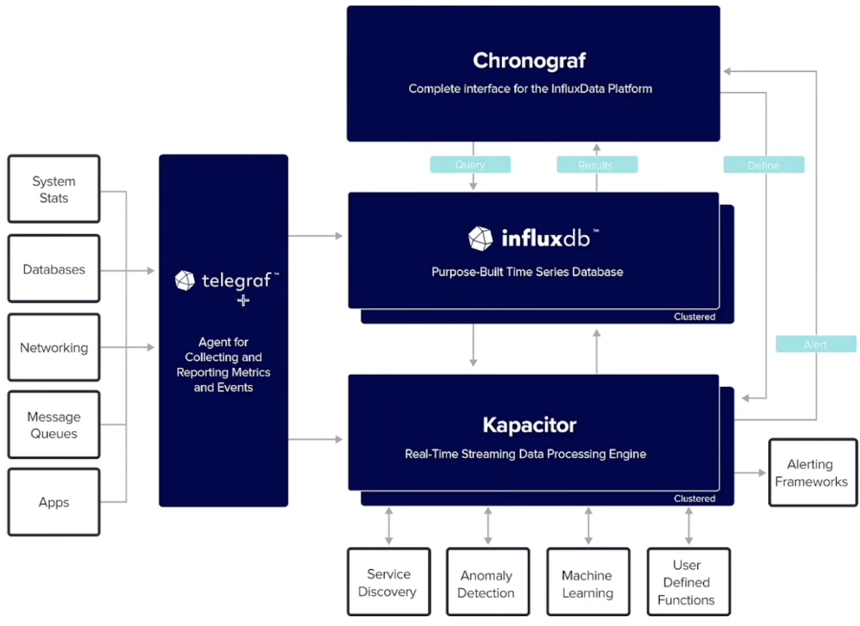
- A popular, open-source TSDB written in Go, designed from the ground up exclusively for time-series data
- Philosophy: Performance through specialization. Provides a complete platform via the TICK Stack
Telegraph- Lightweight, plugin-based agent that collects metrics (system, APIS, StatsD, Kafka, etc.) and forwards them to backends like InfluxDB, Kafka, DatadogInfluxDB- High-performance time-series database optimized for high write throughput, fast time-range queries, an automatic data retentionChronograf- Web UI for visualizing metrics, managing dashboards, and configuring alerts for InfluxDB dataKapacitor- Stream and batch processing engine for InfluxDB data used to detect anomalies, apply custom logic based trigger alerts or actions
- Data Model:
- Measurement: A logical grouping, like an SQL table (e.g.,
cpu_usage). - Tags: Indexed key-value pairs for metadata (e.g.,
host=server-1,region=us-west). Used forWHEREclauses - Fields: Non-Indexed key-value pairs for the actual values(e.g.,
value=45.2) - Timestamp: The time of the measurement
- Measurement: A logical grouping, like an SQL table (e.g.,
Q Why tags and fields are different ?
A Tags are indexed and fields are not, as it’s unnecessary and generally indexes are expensive and if we put high cardinality data in tags the index will explode
Here the cardinality means the number of unique values, so we need to index on the field which have less cardinality it means something like host name would be a good thing to index on rather indexing on user id which have very high cardinality and need to re-index very frequently
High Level Architecture of InfluxDB:
There are two types of storage in InfluxDB
- Catalog
- This is used to store the metadata and in a Postgres-compatible database(RDS/PostgreSQL)
- It functions as cluster’s brain, that tracks databases, tables, columns and file locations
- This updates strictly when files are persisted or deleted
- Object Storage
- This is used to store the actual data in something like S3, Azure Blob, GCS
- It functions as the persistence layer. It stores actual time-series data exclusively as Parquet files
- It has infinite retention at the cost of commodity cloud storage
- This gives us infinite scalability with no reliance on expensive, local attaches SSDs for long-term retention
There are 4 components of Influx DB
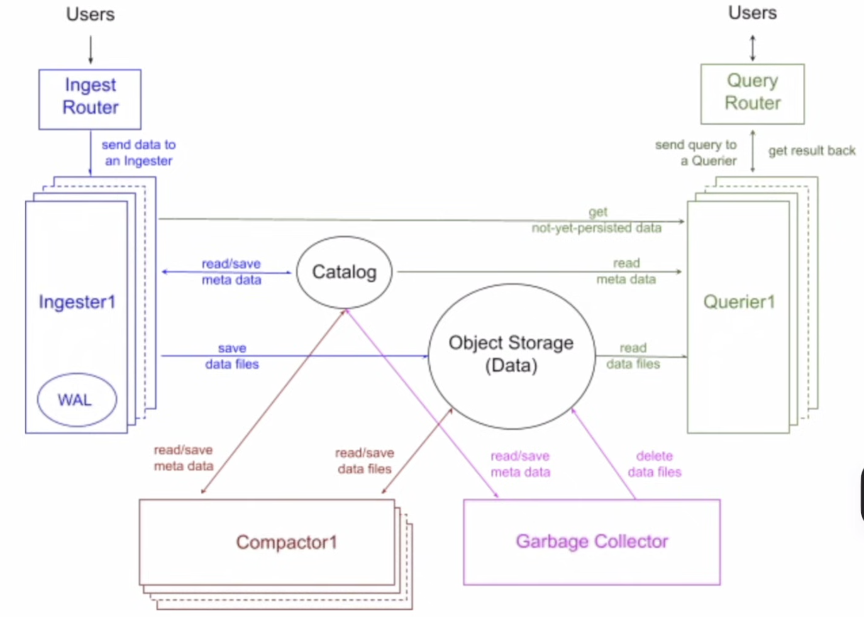
- Ingesters
- It does the data ingestion(write path)
- After data is uploaded to the cloud as parquet files, these are optimized storage via sort-merge and compression
- Ingesters buffer data and build a sort plan using DataFusion
- Sorting by low-cardinality columns maximizes Run-length Encoding(RLE)
- Once written to S3, the Catalog service is updated to make data visible for Compacters and Queries Service
- Compacters
- In this step we turn many small files into fewer and efficient files
- But as these small files increased and being stored in Object storage this increases the I/O during query time, which reduces the query performance. To solve this problem we’ve a data compaction job running in the background which merge the Non-overlapping files into big files which are read optimized
- In short, the compactor reads the newly ingested parquet files, merges them using DataFusion operators, creates larger files and updates the Catalog
- Queries
- User sends and SQL/InfluxQL query and this goes via an
Querier(stateless compute), which calculates the query, resolve it and returns the result - Here is the process of Querier
- Look out for the Tables in the cached Metadata from catalog, if not present do cache refresh
- Read the Metadata and get the tables schema that needed to be queried
- Read the data from the WAL(Injectors - Hot data) and get the data that required for the current query
- Build and execute the query with an optimized query plan
- User sends and SQL/InfluxQL query and this goes via an
- Garbage Lifecycle
- The data in InfluxDB is stored in parquet files which will be present in object storage thus the Deletion happens in two phases
- Soft Delete - Marked as deleted in Catalog, which makes it invisible to queries immediately when triggered by compaction or retention policy
- Hard Delete - Background GC job physically removes file from S3 and clears metadata row
- This is decoupled clean-up process from query/write performance, and no table is locked when GC is running
- The data in InfluxDB is stored in parquet files which will be present in object storage thus the Deletion happens in two phases