Introduction
Turbopuffer is a fast search engine that combines vector and full-text search using object storage, making all your data easily searchable
The system caches only actively searched data while keeping the rest in low-cost object storage, offering competitive pricing. Cold queries for 1 million vectors take p90=444ms, while warm queries are just p50=8ms. This architecture means it’s as fast as in-memory search engines when cached, but far cheaper to run
V1 - Turbopuffer is a search engine - User throws the vectors to the turbopuffer and the turbopuffer cluster them all wrt there similarity and attach it to a cluster and keep all these clusters(cluster1.bin, cluster2.bin,…) in an S3 namespace and it also make a index cluster with name cluster.bin which stores the which cluster have which similarity
V2 - It’s a database which is good at being a search engine - In V1 we have naive S3 implementation where we do 2 round trips. V2 uses LSM(Log-Structured Tree)
earlier we use to do two round trips - get the file via index, then get the content of the file
here we do three round trips
- get the cluster in which the data is present from an index file like cluster.bin
- next trip is to go to that file and get the index block(32-64kB)
- next trip is to go to that index block and get the required vectors
here we do trips because, we get the data, go back calculate which part of these data i need to return,…
here in case of caching we use ring buffer, it means we have a fixed size cache, and we write the cache, and when the cache is full we remove the first one and write the new value there
there are tradeoffs for the turbopuffer
- write latency - as they use S3 they’re dependent on S3 for write latency, it’s nearly some 100ms to write, which is orders of magnitude slow than the mysql
- cold queries, when some unexpected things that user needs, it’s takes time to pull off
Turbopuffer was first on cloudflare R2 on top of cloudflare workers, later it’s on GCP because they have compare and swap storage, later they shifted to S3 for metadata layer and now AWS have compare and swap built in
turbopuffer also have there own client which is compatible with the different cloud companies APIs(signing request was a harder problem)
Architecture
The API routes to a cluster of Rust binaries that access your database on object storage
After the first query, the namespace’s documents are cached on NVMe SSD. Subsequent queries are routed to the same query node for cache locality, but any query node can serve queries from any namespace. The first query to a namespace reads object storage directly and is slow (p50=343ms for 1M documents), but subsequent, cached queries to that node are faster (p50=8ms for 1M documents). Many use-cases can send a pre-flight query to warm the cache so the user only ever experiences warm latency
Turbopuffer is a multi-tenant service, which means each ./tpuf binary handles requests for multiple tenants. This keeps costs low. Enterprise customers can be isolated on request either through single-tenancy clusters, or BYOC
                        ╔═ turbopuffer ════════════════════════════╗
╔════════════╗          ║                                          ║░
║            ║░         ║  ┏━━━━━━━━━━━━━━━┓     ┏━━━━━━━━━━━━━━┓  ║░
║   client   ║░───API──▶║  ┃    Memory/    ┃────▶┃    Object    ┃  ║░
║            ║░         ║  ┃   SSD Cache   ┃     ┃ Storage (S3) ┃  ║░
╚════════════╝░         ║  ┗━━━━━━━━━━━━━━━┛     ┗━━━━━━━━━━━━━━┛  ║░
 ░░░░░░░░░░░░░░         ║                                          ║░
                        ╚══════════════════════════════════════════╝░
                         ░░░░░░░░░░░░░░░░░░░░░░░░░░░░░░░░░░░░░░░░░░░░
Each namespace has its own prefix on object storage. Turbopuffer uses a write-ahead log (WAL) to ensure consistency. Every write adds a new file to the WAL directory inside the namespace’s prefix. If a write returns successfully, data is guaranteed to be durably written to object storage. This means high write throughput (~10,000+ vectors/sec), at the cost of high write latency (p50=285ms for 500KB)
Writes occur in windows of 100ms, i.e. if you issue concurrent writes to the same namespace within 100ms, they will be batched into one WAL entry. Each namespace can currently write 1 WAL entry per second. If a new batch is started within one second of the previous one, it will take up to 1 second to commit
                               User Write
                                 ┌─────┐
                                 │█████│
             WAL                 │█████│
 s3://tpuf/{namespace_id}/wal    └──┬──┘
                                    │
                                    │
╔═══════════════════════════════════╬══════════════╗
║┌─────┐ ┌─────┐ ┌─────┐ ┌─────┐ ┌ ─│─ ┐           ║░
║│█████│ │█████│ │█████│ │█████│    ▼              ║░
║│█████│ │█████│ │█████│ │█████│ │     │           ║░
║└─────┘ └─────┘ └─────┘ └─────┘  ─ ─ ─            ║░
║  001     002     003     004     005             ║░
╚══════════════════════════════════════════════════╝░
 ░░░░░░░░░░░░░░░░░░░░░░░░░░░░░░░░░░░░░░░░░░░░░░░░░░░░
After data is committed to the log, it is asynchronously indexed to enable efficient retrieval (■). Any data that has not yet been indexed is still available to search (◈), with a slower exhaustive search of recent data in the log
Turbopuffer provides strong consistency by default, i.e. if you perform a write, a subsequent query will immediately see the write. However, you can configure your queries to be eventually consistent for lower warm latency
Both the approximate nearest neighbor (ANN) index we use for vectors, as well as the inverted BM25 index we use for full-text search have been optimized for object storage to provide good cold latency (~500ms on 1M documents). Additionally, we build exact indexes for metadata filtering
                   ╔══turpuffer region═══════╗      ╔═══Object Storage═════════════════╗
                   ║      ┌────────────────┬─╬─┐    ║ ┏━━Indexing Queue━━━━━━━━━━━━━━┓ ║░
                   ║      │ ./tpuf indexer │ ║░│    ║ ┃■■■■■■■■■                     ┃ ║░
                   ║      └────────────────┘ ║░│    ║ ┗━━━━━━━━━━━━━━━━━━━━━━━━━━━━━━┛ ║░
                   ║      ┌────────────────┐ ║░│    ║ ┏━/{org_id}/{namespace}━━━━━━━━┓ ║░
                   ║      │ ./tpuf indexer │ ║░│    ║ ┃ ┏━/wal━━━━━━━━━━━━━━━━━━━━━┓ ┃ ║░
                   ║      └────────────────┘ ║░└───▶║ ┃ ┃■■■■■■■■■■■■■■■◈◈◈◈       ┃ ┃ ║░
                   ║                         ║░     ║ ┃ ┗━━━━━━━━━━━━━━━━━━━━━━━━━━┛ ┃ ║░
                   ║                         ║░┌───▶║ ┃ ┏━/index━━━━━━━━━━━━━━━━━━━┓ ┃ ║░
                   ║      ┌────────────────┐ ║░│    ║ ┃ ┃■■■■■■■■■■■■■■■           ┃ ┃ ║░
                   ║   ┌─▶│  ./tpuf query  │ ║░│    ║ ┃ ┗━━━━━━━━━━━━━━━━━━━━━━━━━━┛ ┃ ║░
                ┌──╩─┐ │  └────────────────┘ ║░│    ║ ┗━━━━━━━━━━━━━━━━━━━━━━━━━━━━━━┛ ║░
╔══════════╗    │    │ │  ┌────────────────┐ ║░│    ╚══════════════════════════════════╝░
║  Client  ║───▶│ LB │─┼─▶│  ./tpuf query  │─╬─┘     ░░░░░░░░░░░░░░░░░░░░░░░░░░░░░░░░░░░░
╚══════════╝░   │    │ │  └────────────────┘ ║░
 ░░░░░░░░░░░░   └──╦─┘ │  ┌────────────────┐ ║░
                   ║   └─▶│  ./tpuf query  │ ║░
                   ║      └────────────────┘ ║░
                   ║                         ║░
                   ╚═════════════════════════╝░
                    ░░░░░░░░░░░░░░░░░░░░░░░░░░░
On a cold query, the centroid index is downloaded from object storage. Once the closest centroids are located, we simply fetch each cluster’s offset in one, massive roundtrip to object storage
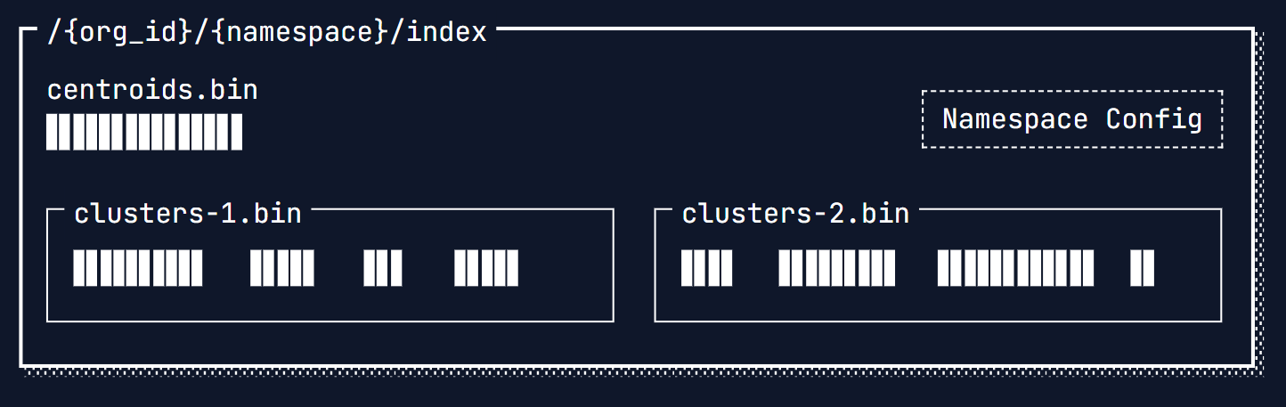 In reality, there are more roundtrips required for Turbopuffer to support consistent writes and work on large indexes. From first principles, each roundtrip to object storage takes ~100ms. The 3-4 required roundtrips for a cold query often take as little as ~400ms
When the namespace is cached in NVME/memory rather than fetched directly from object storage, the query time drops dramatically to p50=8. The roundtrip to object storage for consistency, which we can relax on request for eventually consistent sub 10ms queries
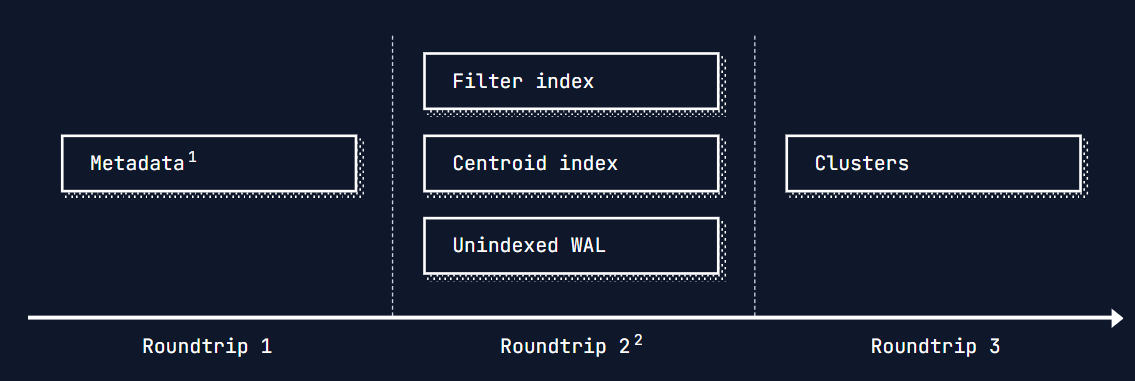
- Metadata is downloaded for the Turbopuffer storage engine. The storage engine is optimized for minimizing roundtrips
- The second roundtrip starts navigating the first level of the indexes. In many cases, only one additional roundtrip is required. But the query planner makes decisions about how to efficiently navigate the indexes. It needs to settle tradeoffs between additional roundtrips and fetching more data in an existing roundtrip
Q What happen Inside Turbopuffer when input vector is given ?
A Turbopuffer is built on Object storage which is AWS S3. When we write a vector in Turbopuffer, a file is created in object storage of WAL, Every new entry makes in, in there and returns an status “ok” when committed to an object storage
- When we commit say 10 vectors it creates a namespace which is nothing but a prefix in S3 and write them onto object store that is literally
file-sync-write - If say the vectors are less (say 10) then we load them all into memory. Like stream them in from S3, then into disc cache and exhaustively walk them into a simple for-loop as it’s cheaper to do it and works really well
- But when we reach to more vectors (say 1,00,000) then we start building the index, so the indexing nodes gets a notification to take that namespace that have prefix on S3, then will start building ANN index
- When we send a read request first it checks the index in the namespace and crawl to the data and give it back, If the index doesn’t exist then it will apply the newest WAL and create an index and mount(WAL) on top of it
- Turbopuffer uses
Centroid Based Index. In this data is in the form of clusters and every cluster have a centroid which is average of all the vectors in that cluster. Now we store the centroids in a place and find the top k closets clusters wrt to the search term, and we download all those clusters data and search for vectors in memory. Here we are downloading more data than Graph based Index but it’s fast as we use S3 and cost effective as the whole data is not present in the memory and we use parallelism while downloading and searching. S3 is very good at these Graph Based Indexare faster than Centroid Based Index but for it all the data should be in memory which is costly. In this if we have given a search term then the closest neighbors are attached to it and later on it’s just traversal and to navigate in graph(traversal) every point to point navigation is a round trip and a round trip in memory is fast and extremely slow in SSD. This can be minimized by shrinking which means decreasing diameter of the graph but not much use, it will be still slow- There is a specific way how Turbopuffer store index of the data they use archive format(Alternative to ProtoBuf), specifically rkyv rust project which allow us to write zero copy(Techniques that avoid unnecessary data copying between memory locations), rust data store format
- Turbopuffer also uses cache, like for cold queries the data will come directly from object storages, and for warm queries, data will come from NVME SSDs (Non-Volatile Memory Express - It is a protocol designed to use the PCI Express (PCIe) bus to connect SSD Solid-State Drive)
Example: Design an search engine for Youtube videos(say playlist search for a youtuber)
- Decide what data is going in it, We can ingest a whole youtube playlist(say 100 videos), but it is difficult to represent the entire episode in 1024 dimensional space, it works and very cheap like it take 100 vectors and 6KB space, can be just done in browser no need of WASM too, but search is not gonna be great. Rather we can take 30secs of video(hard clipped) and store them as vectors, If say a video of 60mins then it takes
100 * 120(1hr/30sec) * 1024(dimensions) * 4(byte integers) = 50MB of data. Which is also pretty small and search is good enough in terms of both quality and search, btw can also do it In-Memory as the size is small - If the size of data increases, supposed if it goes into Gigabytes then we build an approximate neighbor index, called ANN. In this we use KNN and search all the other vectors in O(N) and finding the top results, here we have a trade off of quality for speed. Thus we create a cluster of the data like similar topics in the videos becomes a cluster and we search in specific clusters rather than whole vector search
- It’s also good but, when we are doing ANN on clusters, It is not optimized as our target is to get 95% recall on every search, by doing in clusters we search only around approximately 50% of vectors in the cluster. In this situation we opt different techniques wrt different scenarios, like
- Fine tune the vector search algorithm wrt data
- Use two layers, one index to execute where clause and another index to execute search
- Use conditional searching like, if it cuts off more than 70% of data, search again and this time consider more cluster than before
- Turbopuffer have a fleet of nodes which runs a exhaustive searches against ANN queries to see what actual recall is and inside the
Datadogthey have group by all the different organizations of what there actual recall is, and wrt that they tune the indexes of the clusters and ship the changes to maintain high quality bar
Q How did Turbopuffer build an Vector DB on top of an object storage (AWS S3), how they handled data layer, caching all of that stuff ?
A First Let’s Design a simple Database on AWS S3
- First Create a WAL for the Database, thus create a file per user with a Identifiable prefix and just append the storage names and the actions that took place on the storage, in some format, consider JSON for example
{
  "wal_version": "1.0",
  "created_at": "2025-08-06T08:16:12.543283",
  "namespace_prefix": "s3://turbopuffer-data/",
  "sequence_number": 12345,
  "operations": [
    {
      "operation_id": "8b19fafa-a307-45c9-a04f-c0dcdc6e23f7",
      "timestamp": "2025-08-06T08:16:12.543039",
      "operation_type": "UPSERT",
      "namespace_id": "user_123",
      "batch_id": "batch_001",
      "vectors": [
        {
          "id": "doc_001",
          "vector": [0.1, 0.2, 0.3, 0.4, 0.5],
          "metadata": {
            "title": "Sample Document 1",
            "category": "tech",
            "created_at": "2025-01-01T00:00:00Z"
          }
        },
        {
          "id": "doc_002",
          "vector": [0.6, 0.7, 0.8, 0.9, 1.0],
          "metadata": {
            "title": "Sample Document 2",
            "category": "science",
            "created_at": "2025-01-02T00:00:00Z"
          }
        }
      ]
    },
    {
      "operation_id": "0dc1b0d0-6461-4e31-a597-d6e9e04a7670",
      "timestamp": "2025-08-06T08:16:12.543094",
      "operation_type": "DELETE",
      "namespace_id": "user_123",
      "batch_id": "batch_002",
      "delete_ids": ["doc_003", "doc_004"]
    }
  ],
  "checksum": "sha256:abcd1234...",
  "committed": true
}- Btw you can also do time travel as everything is in the WAL, also no need to do external things as AWS by default provide high availability and durability
Now Let’s Optimize it, to the scale of Turbopuffer
- Why are we using WAL, rather than writing directly to object storage as it’s overhead to manage the WAL in a Structure → Let’s take a step back and think, If we are storing everything in object storge directly and if user runs a query like
SELECT * FROM users WHERE email="example@gmail.com"then the scale of data you need to bring in memory to search is humongous, and also you need scan whole because it might be upserted multiple times, rather we can cache the entries in WAL and search them via indexes in the particular entries - How to handle multiple writer conflicts
- One we can only allow a write at a time → works, but bad idea
- We can add lock service, like when writing to a WAL, we go to a consensus layer like Rafd or Zookeeper and ask permission to write to the WAL and write to the WAL
- Pre-Checks like, keep all the writes in sequence in WAL and only execute the write if the previous sequence number doesn’t have the data, If it does, reject the write
- How often do we push the data from WAL to S3 → Some double digit batches per second will get committed into S3
- How can we do effective search in object storage → We store the B+ Tree with the Data in S3 and when we are searching we search the up-to-date B+ Tree → As these B+ trees be long and there size increases we use LSM(Log-Structured Merge-tree), these are append only logs which help us to do effective writes
- Why we won’t separate both read and write writers → It makes sense to separate them in normal database, but in Vector Database as we read with the same writer we wrote with and they will be warm
Q Whatever I’m Ingesting in Turbopuffer is basically Embeddings, how to i convert back the embeddings in something meaningful ?
A Embeddings are one-way, lossy representations of your data. Turbopuffer does not provide (or need) a “decode” function. Instead, you make the vectors useful by storing the original text / metadata alongside each vector at write-time and returning those attributes at query-time. Attempting to reconstruct the text directly from the embedding is either impossible or requires specialized research models and yields only approximate results. If you think It’s a lot to store the text data with vectors, the just store the database Id of the data along side with vector
Continuous Recall Measurement
All vector databases make a fundamental trade-off between query latency and accuracy. Because what’s not measured is not guaranteed, Turbopuffer automatically samples 1% of all queries to measure the accuracy of the vector index in production (recall). The automatic measurement results are continuously monitored by the Turbopuffer team. Let’s dig into why continuous recall measurement is paramount for any database that offers vector search
For vector search, the naive approach is to exhaustively compare the query vector with every vector in the corpus. The query latency of this approach breaks down when you search 100,000+ vectors
To reduce query latency, search engines use approximate nearest-neighbor (ANN) indexes (such as HNSW, DiskANN, SPANN) to avoid exhaustively searching the entire corpus on each query. For the simplest type of index (inverted index), we can expect a ballpark of sqrt(sqrt(n)) * sqrt(n) * q vectors searched per query, where q is a tunable to make an accuracy/performance trade-off
Some napkin math ballparks (~3 GiB/s SSD) comparing exhaustive and ANN performance on 1536-dimensional f32 vectors:
| Vectors | Exhaustive (SSD) | ANN (SSD) |
|---|---|---|
| 1K | 2 ms | 0.3 ms |
| 10K | 20 ms | 2 ms |
| 100K | 200 ms | 10 ms |
| 1M | 2 s | 60 ms |
| 10M | 20 s | 350 ms |
| 100M | 3.5 min | 2 s |
| 1B | 0.5 h | 10 s |
However, approximate nearest-neighbor algorithms come at the cost of accuracy. The faster you make the query (smaller q), the less the approximate results resemble the exact results returned from an exhaustive search | ||
To evaluate the accuracy of our queries, we use a metric known as recall. Within the context of vector search, recall is defined as the ratio of results returned by approximate nearest-neighbor algorithms that also appear in the exhaustive results, i.e. their overlap. More specifically, we use a metric known as recall@k, which considers the top k results from each result set. For example, recall@5 in the below example is 0.8, because within the top 5 results, 4/5 of the ANN results appear in the exhaustive results |
             ANN                                          Exact
┌────────────────────────────┐               ┌────────────────────────────┐
│id: 9, score: 0.12          │▒              │id: 9, score: 0.12          │▒
├────────────────────────────┤▒              ├────────────────────────────┤▒
│id: 2, score: 0.18          │▒              │id: 2, score: 0.18          │▒
├────────────────────────────┤▒              ├────────────────────────────┤▒
│id: 8, score: 0.29          │▒              │id: 8, score: 0.29          │▒
┌────────────────────────────┤▒              ├────────────────────────────┤▒
│id: 1, score: 0.55          │▒              │id: 1, score: 0.55          │▒
┣─━─━─━─━─━─━─━─━─━─━─━─━─━─━┘▒   Mismatch   ┣─━─━─━─━─━─━─━─━─━─━─━─━─━─━┘▒
 id: 0, score: 0.90          ┃▒◀─────────────▶ id: 4, score: 0.85         ┃▒
┗ ━ ━ ━ ━ ━ ━ ━ ━ ━ ━ ━ ━ ━ ━ ▒              ┗ ━ ━ ━ ━ ━ ━ ━ ━ ━ ━ ━ ━ ━ ━ ▒
 ▒▒▒▒▒▒▒▒▒▒▒▒▒▒▒▒▒▒▒▒▒▒▒▒▒▒▒▒▒▒               ▒▒▒▒▒▒▒▒▒▒▒▒▒▒▒▒▒▒▒▒▒▒▒▒▒▒▒▒▒▒
To ensure Turbopuffer meets 90-95% recall@10 for all queries (including filtered queries, which are much harder to achieve high recall on) Turbopuffer measures recall on 1% of live query traffic and has monitors in place to ensure recall stays above their pre-defined thresholds. 90-95% recall@10 is a good balance of performance and accuracy for most workloads
Native Filtering for high-recall vector search
Vector indexes are often evaluated on recall (correctness) vs latency benchmarks without any filtering, however, most production search queries have a WHERE condition. This significantly increases the difficulty of achieving high recall. Rather than pre-filtering or post-filtering, Turbopuffer uses native filtering to achieve performant high recall queries
Intro: Vector search without filters
The goal of a vector index is to solve the Approximate Nearest Neighbors problem (ANN)
There are many kinds of vector indexes. The two most popular kinds are graph-based and clustering-based indexes
A graph-based index avoids exhaustively searching all the vectors in the database by building a neighborhood graph among the vectors and greedily searching a path in that graph
A clustering-based index groups nearby points together and speeds up queries by only considering clusters whose center is closest to the input vector
|---------------------------|---------------------------|
|                           |                           |
|    x---------x            |    0         1            |
|    |          \           |                           |
|    x---x-------x--x       |    0   0       1  1       |
|     \ /        |   \      |                           |
|      x         x----x     |      0         1    1     |
|     / \       /           |                           |
|    x   \     /            |    0                      |
|         \   /             |                           |
|          \ /              |                           |
|           x---x           |           2   2           |
|           |               |                           |
|           x               |           2               |
|                           |                           |
|                           |                           |
|    Graph-based index      |  Clustering-based index   |
|---------------------------|---------------------------|
In Turbopuffer we use a clustering-based index inspired by SPFresh. The main advantage of this index is that it can be incrementally updated. As documents are inserted, overwritten and deleted, the size of each cluster changes, but the SPFresh algorithm dynamically splits and merges clusters to maintain balance. Because the index is self-balancing, it doesn’t need to be periodically rebuilt, which allows us to scale to very large namespaces
The search algorithm roughly boils down to:
- Find the nearest clusters
- Evaluate all candidates from those clusters The simplicity of this two step process is very convenient for Turbopuffer because if the SSD cache is completely cold, we need to do at most 2 round-trips to object storage to run a query. This is opposed to graph-based ANN structures that would easily require a dozen or more roundtrips.
Vector search + filters != filtered vector search
Consider the use case of semantically searching over a codebase. You may want to search for the top 10 most relevant files within foo/src/*
|-----------------------------------------------------|
|        -                                            |
|                                                     |
|           -         -                               |
|  -                                                  |
|     -                -                              |
|                 -           -                       |
|         Q       -         -                         |
|                                                     |
|                             -                  +    |
|     -                                               |
|                        -                            |
|                           -                  +      |
|                                            +        |
|                                     +        +      |
|                                            +        |
|                                      +              |
|                                                     |
|-----------------------------------------------------|
| legend:                                             |
|  Q:  query vector                                   |
|  +:  document matching the filter                   |
|  -:  document not matching the filter               |
|-----------------------------------------------------|
The diagram above illustrates this problem, simplified to 2 vector dimensions and a small number of documents (typically the number of dimensions is 256 - 3072 and the number of documents is 0-1B+)
Assume we have some sort of vector index and some sort of attribute index (e.g. B-Tree) on the path column. With only these indexes to work with, the query planner has two choices: either pre-filter or post-filter
A pre-filter plan works as follows:
- Find all documents that match the filter
- Compute the distance to each one
- Return the nearest k
This plan would achieve 100% recall, but notice that step (2) doesn’t actually use the vector index. Because of that, the cost of this plan is O(dimensions * matches). That’s too slow
A post-filter plan works as follows:
- Find the 10 approximate nearest neighbors to Q
- Filter the results
This is much faster because it uses the vector index. But as shown in the diagram, none of the nearest 10 documents match the filter! So the recall would be 0%, no matter how well the vector index performs on unfiltered queries
So the pre-filter and post-filter plans are both bad. We want >90% recall with good latency, and that’s not achievable with query planner hacks unless the vector and the filtering indexes cooperate with each other
| planner    | recall | perf |
|------------|--------|------|
| postfilter |     0% | 20ms |
| prefilter  |   100% | 10s  |
| target     |    90% | 25ms |
Native filtering
The goal of the query planner is that no matter what kind of filters we have, the number of candidates considered remains roughly the same as it would be for an unfiltered query
To achieve this goal we designed our attribute indexes to be aware of the primary vector index, understand the clustering hierarchy and react to any changes (like the SPFresh rebalancing operations). This allows us to extract much more information from these indexes, and use them at every step of the vector search process. The resulting query plan is:
- Find the nearest clusters that contain at least one match
- Evaluate matching candidates from those clusters
The diagram below shows the same dataset as before. We can scan the "foo/src/*" range in the attribute index to see that all the matching results are in clusters 4 and 5, allowing us to skip clusters 0, 1, 2, 3, even though they are closer to the query point
|-----------------------------------------------------|
| vector index:                                       |
|                                                     |
|        0                                            |
|                                                     |
|           0         1                               |
|  0                                                  |
|     0                1                              |
|                 1           3                       |
|         Q       1         3                         |
|                                                     |
|                             3                  4    |
|      2                                              |
|                         3                           |
|                            3                  5     |
|                                             5       |
|                                     5         5     |
|                                             5       |
|                                       5             |
|                                                     |
|-----------------------------------------------------|
| attribute indexes:                                  |
|   path=foo/readme.md -> [0, 1]                      |
|   path=foo/src/main.rs -> [5]                       |
|   path=foo/src/bar.rs -> [4, 5]                     |
|   ...                                               |
|-----------------------------------------------------|
| legend:                                             |
|  Q:  query vector                                   |
|  0:  document in cluster 0                          |
|  1:  document in cluster 1                          |
|      ...                                            |
|  i:  document in cluster i                          |
|-----------------------------------------------------|
Implementation
The query filter can be a complicated nested expression involving And, Or, Eq, Glob, and other operators applied over one or more attributes. The attribute indexes need to quickly convert these filters to data relevant to vector search, like:
- the set of relevant clusters
- (if needed) the number of matches in each cluster
- (if needed) the exact bitmap of matches within a cluster
Retrieval is an old problem with lots of existing research. The only tpuf-specific aspects of it are:
- How to tie the attribute index to a vector index
- How to store this index on blob with minimal write amplification
- How to optimize query performance when the SSD cache is cold
The solution to (1) is simple. For each document, the primary vector index assigns an address in the form of {cluster_id}:{local_id}, where local_id is just a small number unique to that cluster. Then the attribute index uses these addresses to refer to documents. When an address changes, the attribute index needs to be updated
Solving problem (2) is important because files on blob storage cannot be partially updated. They can only be fully rewritten. Our LSM tree storage engine allows us to implement partial file updates as key-value overwrites. To avoid fully overwriting the entire index on each update, we use (attribute_value, cluster_id) as the key, and Set<local_id> as the value in the LSM
To solve problem (3) we need to ensure that the data needed to execute the filter can be downloaded from s3 quickly, and that the number of roundtrips required to run the filter is small. To keep index size small, we compress the Set<local_id> values as bitmaps. Additionally, we pre-compute a downsampled version of each index to cluster granularity, which allows us to perform bitmap unions and intersections on the cluster level before fetching exact bitmaps (if at all needed). This two-step process also limits the number of blob storage round-trips on a completely cold query
|-----------------------------------------------------|
| row-level attribute indexes:                        |
|   path=foo/readme.md -> [0:0, 0:1, 1:2]             |
|   path=foo/src/main.rs -> [5:0, 5:1]                |
|   path=foo/src/bar.rs -> [4:0, 5:2, 5:3, 5:4]       |
|   ...                                               |
|-----------------------------------------------------|
| cluster-level attribute indexes:                    |
|   path=foo/readme.md -> [0, 1]                      |
|   path=foo/src/main.rs -> [5]                       |
|   path=foo/src/bar.rs -> [4, 5]                     |
|   ...                                               |
|-----------------------------------------------------|
How Cursor Built their Indexing Pipeline ?
Every keystroke we do creates a state deviation for cursor’s on-server index. natively just reindexing the entire codebase is slow and expensive
Cursor uses Merkle trees - for any change, it takes O(log(n)) bandwidth to find where the client/server disagree. Like bloom filters, a Merkle Tree is a data structure where every leaf node stores the hash of a block of data, and every parent stores the hash of its children
- Every file gets a hash, based on its contents. The leaves of the tree are files
- Every folder gets a hash, based on its hash of its children
- Cursor uses Merkle trees at the client level with rust hooks on TS frontend. cursor-client obfuscates(~unclear) files names, and creates Merkle tree based on local files, and after indexing it again creates a Merkle tree on their server-side
- When Cursor starts, a ‘handshake’ occurs. The client sends its root hash to the server
- If the root hashes match, the server knows nothing has changed → Done → Zero data transferred
- If they don’t match, the server-client can quickly compare the hashes of the child nodes to find exactly which branch of the tree is different → They do tree traversals downstream
- Only those changed files are sent to the server to be re-chunked, re-embedded, and updated in Turbopuffer(obj storage vector database)
- Cursor also does an index sync CRON every 10-mins to determine which files need re-indexing. important here to note is that cursor ignores sensitive data(API key, passwords, envs). It respects gitignore and .cursorignore and will not index files listed there
Q For “Code” Indexing, how cursor handle large contexts of the codebase ?
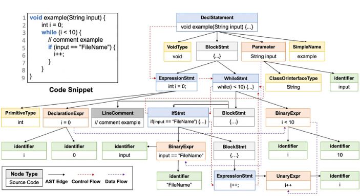
A One solution can be Chunking blocks of code like we do for text (fixed-token length, paragraph-based, etc.) is bad. Code follows a specific syntax and has meaningful units/well-defined structure - classes, methods, and functions
To solve this Cursor uses - Abstract Syntax Trees(AST), and Tree Sitters to store the semantic meaning of the code
 After the chunking of the code is done, cursor creates the embeddings (probably with open Ai’s text-embedding-3-large/custom finetuned embedding model). These embeddings are then stored into Turbopuffer
When a user is actively working on a codebase, its index data is automatically moved to this cache. This ensures that while the entire dataset lives on low-cost storage, active queries are served with low latency
Q Why not use native Postgres or MySQL vector databases ?
A There are a set of reasons
- Postgres will some times make a naive decision of not having a query planner that’s completely integrated into the high recall use cases, we can solve this by looking at more data or pre filtering
- Also when the data is huge means vectors are large then they do not compress well, and if we use postgres then we store the data in one write replica and some read replicas and this need us to buy more disc space as at least we only use 50% of disc space, and managing them is a nightmare. but when we use objects storage like S3 which Turbopuffer uses internally, we can easily replicate and distribute across the globe