Elliptic Curve Cryptography

“It is possible to write endlessly on elliptic curves” ~ Serge Lang
Elliptic curves powers about 70% of TLS exchanges(https) as of 2022

Diophantine Equations (Historical Motivation)

Q What Are Diophantine Equations?
A Diophantine equations are polynomial equations where we do not look for real or complex solutions. Instead, we restrict ourselves to Integers ($\mathbb{Z}$), or Rational numbers ($\mathbb{Q}$). This restriction makes the problem much harder
A famous example is:

$$X^n+Y^n=Z^n,X,Y,Z\in \mathbb{Z}$$

This equation asks: “Can three whole numbers raised to the same power ever add up like this?”
An equivalent way to write this is:

$$x^n+y^n=1,x,y\in \mathbb{Q}$$

This second form is often easier to analyze because it reduces the number of variables

Q Why Are Diophantine Equations Hard?
A The difficulty comes from where we are searching for solutions

• Over $\mathbb{R}$ or $\mathbb{C}$:
  • We can draw graphs
  • Use calculus
  • Use approximation methods
  • Solutions are usually easy to find
• Over $\mathbb{Z}$ or $\mathbb{Q}$:
  • No smooth structure
  • No approximation
  • Solutions may be extremely sparse or not exist at all

A small change in the allowed number system completely changes the problem. Famous Example: Fermat’s Last Theorem he claimed that:

$$X^n+Y^n=Z^n$$

has no integer solutions for $n>2$
This statement took over 350 years to prove and was finally proved by Andrew Wiles which uses deep ideas from elliptic curves. This shows how difficult Diophantine equations can be

Limits of Computation (Hilbert’s 10th Problem)

One might hope for a general algorithm:

Input any Diophantine equation → Output whether it has solutions

Unfortunately, this is impossible

It was proven that:

• There is no algorithm
• No finite procedure
• That works for all Diophantine equations

This problem is undecidable

This result tells us something deep:

Mathematics has fundamental limits, just like computation

Q What do we want to know?
A For a given Diophantine equation, we usually ask:

1. Does a solution exist at all?
2. If it exists, how many solutions are there?
   • None
   • A finite number
   • Infinitely many

Since the general case is impossible, we focus on simpler classes of equations

One Variable Case

Consider a polynomial equation with one variable:

$$a_n{x}^n+a_{n-1}{x}^{n-1}+\cdots +a_{1}x+a_0=0$$

This is the simplest possible Diophantine equation
Surprisingly, this case is completely solvable

Rational Root Theorem (Gauss’ Lemma)

Statement: If a rational number $\frac{p}{q}$ (in lowest terms) is a solution, then:

• $p$ divides the constant term $a_0$
• $q$ divides the leading coefficient $a_n$

This Helps as instead of searching infinitely many rationals:

• We get a finite list of candidates
• Each candidate can be checked directly

Example (Intuition) Suppose:

$$2x^2+3x-2=0$$

Possible values:

• Numerator divides $-2$: $\pm 1,\pm 2$
• Denominator divides $2$: $\pm 1,\pm 2$
• So only a small list needs to be tested

Conclusion:

• One-variable Diophantine equations are decidable
• We can always determine whether rational or integer solutions exist

Linear Equations in Two Variables

Consider:

$$ax+by=c$$

Rational Solutions: This equation represents a line

• Any line (except vertical ones) contains infinitely many rational points
• You can always parameterize the solutions

So:

Linear equations in two variables always have infinitely many rational solutions

Integer Solutions: Integers are more restrictive than rationals
Theorem:

• If $\gcd (a,b)\nmid c$, then no integer solutions exist
• If $\gcd (a,b)\mid c$, then infinitely many integer solutions exist

Q Why This Works (Intuition) ?
A

• Any integer combination $ax+by$ must be divisible by $\gcd (a,b)$
• If $c$ is not divisible by this gcd, equality is impossible
• Example

$$4x+6y=5$$

$\gcd (4,6)=2$, but $2\nmid 5$ → no solutions

Quadratic Equations in Two Variables (Conics)

General form:

$$a{x}^2+bxy+c{y}^2+dx+ey+f=0$$

Circle, Ellipse, Hyperbola describe conic sections
Now let’s understand, Geometry of Rational Points
If we know one rational point on the curve:

• Draw a line through it with rational slope
• The second intersection point must also be rational
• Repeating this generates all rational points

Q Do Rational Points Exist?
A Finding the first rational point is the hard part

• Hasse Principle (Local-to-Global)
  • A conic has a rational solution if and only if:
    • It has a solution over the real numbers, and
    • It has a solution modulo $p^k$ for every prime $p$
  • Why this is important
    • Real solutions check global geometry
      • Solving an equation over the real numbers answers a very basic question “Does the curve actually exist as a geometric object?”
      • For example:

$$x^2+y^2=-1$$

		- This equation has: No real solutions, No rational solutions, No integer solutions. Because the left-hand side is always non-negative over the reals. If there is no real point, then there is no “shape” to study
		- So checking real solutions tells us:
			- Whether the curve is _geometrically possible_
			- Whether it has any points at all in ordinary space
		- If an equation fails over $\mathbb{R}$, there is no need to check anything else
	- $p$-adic solutions check arithmetic consistency
		- Even if an equation has real solutions, it might still fail for number-theoretic reasons
		- To detect this, we check solutions modulo primes 
		- What Does “$p$-adic” Mean (Intuitively)?
			- Instead of asking: "Does the equation have a solution exactly?"
			- We ask: "Does it have solutions _approximately_ modulo powers of a prime?"
			- For example, we check: Mod $2$, Mod $4$, Mod $8$, Mod $p^k$ for every prime $p$
			- If an equation fails modulo some prime power, then:
				- It cannot have an exact rational solution
				- Because rationals must reduce consistently modulo every prime
		-  Example of Arithmetic Obstruction, consider:

$$x^2\equiv -1(\mathrm{mod}4)$$

		- This has no solution, because:
			- Squares modulo 4 are only $0$ or $1$
			- Never $-1 \equiv 3$
		- So any equation forcing this condition cannot have a rational solution, even if it has real solutions
		- Thus, $p$-adic checks detect hidden arithmetic impossibilities
	- Together, they guarantee a rational solution
- This gives us a practical decision method

Q What Does “Local to Global” Mean?
A The phrase local to global describes a general strategy in mathematics:

If a problem can be solved locally everywhere,
then it can be solved globally

• Global: The Full, Exact Solution
  • A solution over the rational numbers $\mathbb{Q}$ (or integers)
  • An exact solution, not approximate
  • One solution that works everywhere at once
  • For example:

$$x^2+y^2=5$$

- A global (rational) solution is:

$$(x,y)=(1,2)$$

- This single solution works in the full number system

• Local: Checking the Problem in Pieces
  • A local solution means checking the equation in simpler or “partial” settings
  • Instead of solving the equation outright, we ask: “Does the equation make sense when viewed from a limited perspective?”
  • There are two main local perspectives
    1. Local at Infinity: Real Numbers
       • Checking solutions over Real Numbers, this answers: “Does the equation have any geometric meaning at all?”
       • If there are no real solutions, then:
         • There cannot be rational or integer solutions
         • The problem fails globally
    2. Local at Each Prime: Modulo Arithmetic ($p$-adic)
       • For each prime $p$, we check whether the equation has solutions Modulo $p$, Modulo $p^2$, Modulo $p^3$, And so on
       • This checks: “Is the equation arithmetically consistent with respect to prime factorizations?”
       • If it fails for even one prime, then “A global rational solution is impossible”
• Local-to-Global Principle (Informal): A local-to-global principle says

If an equation has a solution: Over the reals, and Over ${\mathbb{Q}}_p$ for every prime $p$ then it has a rational solution

• This is exactly what happens for conics, this local to global works for Linear and Quadratic (conics) but will not work for Cubic (elliptic curves)

Cubic Equations and Elliptic Curves

General cubic:

$$a{x}^3+b{x}^{2}y+cx{y}^2+d{y}^3+e{x}^2+fxy+g{y}^2+hx+iy+j=0$$

These equations define elliptic curves

Mordell’s Theorem:
If an elliptic curve

• Has no singularities (no cusps or crossings)
• Has at least one rational point

Then:

All rational points form a finitely generated group

Q What This Means (Intuition)?
A

• There may be infinitely many rational points
• But they all come from finitely many generators
• Similar to how all integers come from repeated addition of 1

Q What Fails Compared to Quadratics ?
A

• No local-to-global principle
• A curve may have solutions everywhere locally but none globally

This makes elliptic curves much harder

Note:

• Ellipses → degree 2
• Elliptic curves → degree 3

They are not the same object, despite the name. The name comes from elliptic integrals, which appear when computing the arc length of an ellipse
These integrals involve expressions like:

$$y=\sqrt{P_3(x)}$$

Squaring both sides produces cubic equations similar to elliptic curves

Checkpoint 1:

• Diophantine equations are easy over $\mathbb{R}$, hard over $\mathbb{Z}$ and $\mathbb{Q}$
• One-variable equations are completely solvable
• Linear equations are easy
• Quadratic equations are solvable using geometry and the Hasse principle
• Cubic equations lead to elliptic curves: - Finite generation (Mordell) - No local-to-global principle - Deep mathematical structure

Mathematical Background

Fields

A field $K$ is a set with two operations ($+$) and ($\cdot$) such that:

• $(K,+)$ is an abelian group with identity $0$
• $(K\setminus \{0\},\cdot )$ is an abelian group with identity $1$
• Distributive law: a(b + c) = ab + ac
• 0 $\ne$ 1
• This means, Informally Add, Subtract, Multiply, Divide (by non-zero elements)

Structure	Field?
$\mathbb{Q}$	✅
$\mathbb{R}$	✅
$\mathbb{Z}$	❌ (no division)
$\mathbb{Z}/p\mathbb{Z}$	✅ if $p$ is prime

Finite Fields

Cryptography mostly uses finite fields, because:

• Elements have fixed size
• Efficient storage
• Efficient arithmetic

Classification Theorem:
For every prime $p$ and every $n\in {\mathbb{Z}}^{+}$: (see example to understand better)

• There exists a unique field of size $p^n$
• Denoted:

$${\mathbb{F}}_{p^n}\text{or}GF(p^n)$$

- If $n = 1$:

$${\mathbb{F}}_p=\mathbb{Z}/p\mathbb{Z}$$

- If $n > 1$:

$${\mathbb{F}}_{p^n}=\frac{{\mathbb{F}}_p[X]}{(f(X))}$$

Where: $f(X)$ is an irreducible polynomial of degree $n$

• Interpretation
  • Elements are polynomials of degree < $n$
  • Arithmetic is done modulo $f(X)$
• Example

$${\mathbb{F}}_8={\mathbb{F}}_2[X]/(X^3+X+1)$$

Characteristic of a Field:
The characteristic of a field $\mathbb{F}$ is the smallest $\ell$ such that:

$$\underset{\ell \text{ times}}{\underbrace{1+1+\cdots +1}}=0$$

If no such $\ell$ exists:

$$\text{char}(\mathbb{F})=\infty$$

Field	Characteristic
$\mathbb{R}$	$\infty$
$\mathbb{Q}$	$\infty$
${\mathbb{F}}_{p^n}$	$p$
Important Consequences

1. Fields of different characteristic have no non-trivial homomorphisms
2. Freshman’s Dream holds in characteristic $p$:

$$(x+y{)}^p=x^p+y^p$$

This fails in characteristic 0

Field Extensions

If $k\subseteq K$ are fields: $K$ is a field extension of $k$
Examples:

$$\mathbb{Q}\subset \mathbb{R}\subset \mathbb{C}$$ $${\mathbb{F}}_p\subset {\mathbb{F}}_{p^2}\subset {\mathbb{F}}_{p^3}\subset \overline{{\mathbb{F}}_p}$$

Algebraic Closure

• A field $\overline{K}$ is algebraically closed if: Every polynomial over $K$ has all its roots in $\overline{K}$
• Btw Every field has an algebraic closure
• Key Properties:
  • Algebraic closures are always infinite
  • Finite fields are not algebraically closed
• Approximating Algebraic Closure
  • For finite fields:
    • ${\mathbb{F}}_{p^{n!}}$ contains roots of all polynomials of degree ≤ $n$
    • This gives a finite approximation of the closure

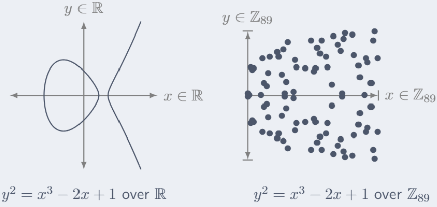
Elliptic Curve Definitions

Elliptic curves arise naturally when studying Diophantine equations of degree 3 in two variables. They form the mathematical foundation of Elliptic Curve Cryptography (ECC) Despite the name, elliptic curves are not ellipses. They are algebraic curves defined by cubic equations, while ellipses are quadratic (degree 2)
A general cubic equation in two variables looks like:

$$a{x}^3+b{x}^{2}y+cx{y}^2+d{y}^3+e{x}^2+fxy+g{y}^2+hx+iy+j=0$$

Using suitable changes of variables, any non-singular cubic curve can be rewritten as:

$$y^2+axy+by=x^3+c{x}^2+dx+e$$

This is called the (general) Weierstrass form
It has two key advantages:

• All cubic behavior is on one side
• The equation is quadratic in “y”

This can be further simplified, if the field “K” satisfies:

$$\mathrm{char}(K)\ne 2,3$$

then the equation simplifies further to:

$$y^2=x^3+ax+b$$

This is the short Weierstrass form
This is useful as it simplifies formulas for Point addition, Discriminant, Invariants
From now on, elliptic curves are assumed to be in short Weierstrass form unless stated otherwise
Elliptic curves can also be represented in other equivalent forms:

• Montgomery Curves
  • Efficient for cryptography
  • Group law uses only x-coordinates
• Edwards Curves
  • Very fast and safe arithmetic
  • Complete addition formulas (no edge cases)
• Legendre Curves
  • Often used in theoretical work

All these are isomorphic to Weierstrass curves, they describe the same curve in different coordinates

Definition of an Elliptic Curve:
Let “k” be a field
An elliptic curve over “k” is given by:

$$E:y^2=x^3+ax+b\text{with }a,b\in k$$

Points on an Elliptic Curve
For any field extension (K \supset k), define:

$$E(K)=\{(x,y)\in K^2\mid y^2=x^3+ax+b\}\cup \{\infty \}$$

Here:

• E(K) is the set of all points with coordinates in K
• Infinity is the point at infinity

The point “Infinity” is added for geometric reasons:

• In projective geometry, curves must be closed
• Every line intersects a cubic curve in three points
• “Infinity” acts as the identity element for the group law
• Without “Infinity”, the algebraic structure would break

Discriminant

The discriminant tells us whether the elliptic curve is well-behaved
Let:

$$E:y^2=x^3+ax+b$$

The discriminant of (E) is:

$$\Delta =-16(4a^3+27b^2)$$

Singular vs Non-Singular Curves

• The curve is singular if: $$\Delta =0$$
• Otherwise, the curve is non-singular
• Why This Matters
  • Singular curves have cusps or self-intersections
  • The group law fails on singular curves
  • Elliptic curves must be non-singular

There is an Alternative View Using Roots, Write the equation as:

$$E:y^2=f(x)$$

Let (x_1, x_2, x_3) be the roots of f(x)
Then the discriminant can also be written as:

$$\Delta =(x_1-x_2{)}^2(x_2-x_3{)}^2(x_3-x_1{)}^2$$

Interpretation

• Delta = 0 if two roots coincide
• This means f(x) has a repeated root
• Repeated roots produce singular points
• So: Non-singular curve ⇔ all roots are distinct

j-Invariant

The j-invariant classifies elliptic curves up to isomorphism
For an elliptic curve:

$$E:y^2=x^3+ax+b$$

the j-invariant is defined as:

$$j(E)=-1728\frac{(4a{)}^3}{\Delta }$$

Q Why the j-Invariant Exists ?
A Different equations may describe the same elliptic curve under a change of variables. The j-invariant is a numerical fingerprint:

• Same (j) ⇒ same curve (up to isomorphism)
• Different (j) ⇒ fundamentally different curves

Isomorphisms of Elliptic Curves:
Any isomorphism between curves in short Weierstrass form must be:

$$(x,y)\mapsto (u^{2}x,u^{3}y)$$

where:

$$u\in {\overline{K}}^{\text{*}}$$

This change:

• Preserves the curve structure
• Changes coefficients (a, b)
• Leaves j(E) unchanged

Classification Theorem:
Let (E, E’) be elliptic curves over a field (K) Then:

$$E\cong E^{\prime }\text{ over }\overline{K}⟺j(E)=j(E^{\prime })$$

• Over the algebraic closure, elliptic curves are completely classified by (j)
• The j-invariant determines the curve up to isomorphism

Representation and Group Law

An elliptic curve is given by an equation like:

$$E:y^2=x^3+ax+b$$

We want to define a way to “add” points on the curve so that:

• Adding points behaves like addition in algebra
• We get:
  • an identity element
  • inverses
  • associativity (hardest part)
• This turns the curve into a group
• This “addition” is called the group law

Geometry Behind the Group Law:

1. Intersections of Lines and Curves
   • A line has degree 1
   • An elliptic curve has degree 3
   • It means, A line intersects a cubic curve in exactly 3 points, counting multiplicities and points at infinity
2. We define the group operation so that. Any three points lying on the same straight line add up to zero

$$P+Q+R=\mathcal{O}$$

- where $\mathcal{O}$ = point at infinity (the identity element)
- Why Do We Need the Point at Infinity? Consider this situation:
	- Take a point P
	- Draw a vertical line through it
	- This line hits the curve at "P", the point directly opposite across the x-axis, nothing else in the finite plane - But we _must_ have three intersection points  
	- The solution is we add a special point called the point at infinity called "O"
- This point is not visible on the graph and it acts as the identity element which makes the geometry consistent

3. Inverses on the Curve - For a point: P = (x, y), its inverse is defined as: -P = (x, -y)
- Why does this make sense? In a vertical line through x intersects the curve at (x, y), (x, -y), O. So P + (-P) = O. so this is why we want from inverses in a group 4. Adding Two Distinct Points P + Q. Let:

$$P_1=(x_1,y_1),P_2=(x_2,y_2)$$

- Draw the line through `P_1` and `P_2`
- This line intersects the curve at a third point
- Reflect that third point across the x-axis
- The reflected point is `P_1` + `P_2`

5. Special Cases - Case 1: Opposite Points - If:

$$x_1=x_2\text{and}{y}_1=-y_2$$

	- Then:  

$$P_1+P_2=\mathcal{O}$$

- Case 2: Identity Element
	- If:
		- `P_1 = O`, then `P_1 + P_2 = P_2`
		- `P_2 = O`, then `P_1 + P_2 = P_1`
	- This makes "O" behave like zero

Translating Geometry into formulas

• Step 1: Defining the Slope,
  • If points are different (P_1 not equal to P_2):

$$\lambda =\frac{y_2-y_1}{x_2-x_1}$$

- If points are the same (P_1 = P_2):
	- We use the tangent line
	- Why?
		- The tangent counts as two intersections (multiplicity 2)
		- So total intersections = 3
	- The slope is:

$$\lambda =\frac{3x_1^2+a}{2y_1}$$

• Step 2: Compute the New Point
  • Once lambda is known:

$$x_3={\lambda }^2-x_1-x_2$$ $$y_3=\lambda (x_1-x_3)-y_1$$

	Then:

$$P_1+P_2=(x_3,y_3)$$

With these rules, we can get the following group properties:

• Identity: “O”
• Inverses: reflection across x-axis
• Closure: result is always on the curve
• Commutativity: P + Q = Q + P
• Associativity: It is non-trivial and messy to prove, but it does hold, and that’s enough for cryptography

Scalar Multiplication

For ( n > 0 ):

$$[n]P=\underset{n\text{ times}}{\underbrace{P+P+\cdots +P}}$$

Extensions:

• (0)P = O
• (-n)P = (n)

Cryptography relies on:

• Scalar multiplication because it’s easy
• Reversing it (discrete log problem) is hard

For Efficient Computation we use Double-and-Add method
Naively computing (n)P takes O(n) additions, too slow

Instead:

• Use binary representation of n
• Repeatedly:
  • double a point
  • conditionally add
• Complexity: O(logn)

Multiplication-by-(m) Map:
Define a function:

$$[m]:E\to E$$

by:

$$P\mapsto [m]P$$

This is called an endomorphism because Input and output are both on the same curve

Torsion Subgroups:
The m-torsion subgroup is:

$$E[m]=\ker [m]$$

Meaning:

$$E[m]=P\in E\mid [m]P=\mathcal{O}$$

Intuition:

• Points in E[m] have finite order
• Example:
  • Order 2 → point lies in E[2]
  • Order 6 → lies in E[2], E[3], E[6]

Torsion points are especially important over finite fields.

Number of Points on an Elliptic Curve

Let the curve be defined over a finite field F_q
Heuristic Estimate:

• Each x gives at most two values of y
• A random value is a quadratic residue with probability ≈ 1/2
• So we expect:

$$|E\ast ({\mathbb{F}}_q)\approx q+1$$

(+1 for the point at infinity)

Hasse’s Theorem:

$$\left|E\ast ({\mathbb{F}}_q)-(q+1)\right|\le 2\sqrt{q}$$

• The number of points is very close to q + 1
• The error is tightly bounded and this is very precise
• Exact value can be efficiently found using Schoof’s algorithm in O((logq)^8)

Discrete Logarithm(DLP)

Cryptography relies on hardness assumptions

• Proving something is “easy” → just show a solution
• Proving something is “hard” → must show no efficient solution exists
• This is extremely difficult, especially for algorithms

This is similar to:

• NP problems: solutions are easy to verify
• co-NP problems: must prove no solution exists → much harder

Cryptographers cannot prove absolute hardness, so instead they:

• Choose problems with no known efficient algorithms
• Build cryptographic schemes on top of them
• Show: breaking the scheme ⇒ solving the hard problem

This creates a tower of problems. If the base problem is hard, everything built on it is secure

Q What Is a Discrete Logarithm?
A

• In real numbers 2^8 = 256, so log_2(256) = 8 → very easy
• In finite groups, We know P, we know [k]P, we want to find k
• This problem is called the Discrete Logarithm Problem (DLP)
• In finite groups, no efficient algorithm is known

Formal Definition of the Discrete Logarithm Assumption:

1. Group Generation
   • Let $\text{Gen}(1^{\lambda })$ be a probabilistic polynomial-time (PPT) algorithm
   • It outputs a cyclic group: $$\mathbb{G}=(+,P,q)$$ where:
     • $\mathbb{G}=⟨P⟩$
     • $q=|\mathbb{G}|$
2. Adversary Game Definition
   • An attacker “A” is given:
     • The group “G”
     • A random scalar multiple [k]P
   • The attacker tries to recover “k”
   • The advantage of the attacker is defined as:

\mathrm{Adv}^{\mathrm{dlp}}_{\mathcal{A}}(\lambda)

\Pr\left[
\mathcal{A}(1^\lambda, \mathbb{G}, [k]P) = k
\middle| \mathbb{G} \leftarrow \text{Gen}(1^\lambda),
k \leftarrow \mathbb{Z}q
\right]
$3.WesaytheDLPassumptionholdsif:-ForeveryPPTattacker"A"-Theadvantage$ \mathrm{Adv}^{\mathrm{dlp}}{\mathcal{A}}(\lambda)$$ is negligible - This means, Success probability decreases faster than any polynomial - Essentially impossible for large parameters

Q Why DLP Alone Is Not Enough ?
A The DLP assumption is weak. It is hard to use directly and Most cryptographic constructions need stronger assumptions

• So in practice we rely on:
  • Computational Diffie-Hellman (CDH)
    • Given P, [x]P, [y]P then compute [xy]P
    • This is exactly what Diffie–Hellman key exchange needs.
  • Decisional Diffie-Hellman (DDH)
    • Distinguish between:
      • Real tuple: P, [x]P, [y]P, [xy]P
      • Random tuple: P, [x]P, [y]P, [z]P
      • where z is random and this is a decision problem, not a computation problem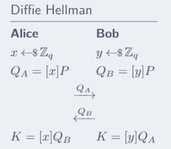
      • 
      • Here in the example we get: K = [x]Q_B = [x][y]P = [xy]P = [y][x]P =[y]QA = K
• Relationship Between Assumptions

$$\text{DDH}{\le }_R\text{CDH}{\le }_R\text{DLP}$$

- If you can solve DLP, you can solve CDH
- If you can solve CDH, you can solve DDH

Note:

1. Pairings make DDH easy on elliptic curves, for example

$$e(g^x,g^y)=e(g,g^z)$$

- So DDH is easy and CDH is still believed hard
- This is why ECC protocols are carefully designed

2. Representation Matters - Two groups may be isomorphic but have very different security, for example - ${\mathbb{Z}}_{p-1}$ (additive) → DLP is trivial - ${\mathbb{F}}_p^{\ast }$ (multiplicative) → DLP is hard - Hardness is NOT preserved by isomorphism

Assumption	Group	Best Known Attack	Approx. Complexity
RSA	${\mathbb{Z}}_N$	Number Field Sieve	$\exp (c\sqrt[3]{\log N})$
DLP	${\mathbb{F}}_p^{\ast }$	Number Field Sieve	$\exp (c\sqrt[3]{\log p})$
DLP	$E({\mathbb{F}}_p)$	Pollard Rho	$\sqrt{p}$
Dangerous Curves

1. Singular Curves
   • They’re Isomorphic to (F_p)^*, these are additive group F_p
   • DLP becomes easy
2. Small Embedding Degree
   • MOV attack maps ECC DLP → finite field DLP
   • If embedding degree is small → security collapses
   • For examples Supersingular curves and Anomalous curves
3. Pairing-Friendly Curves
   • Pairings reduce ECC DLP to finite fields
   • Good for advanced crypto
   • Bad for standard ECDH/ECDSA
4. Curves Over (F_p)^k with Small Factors
   • These are Vulnerable to: GHS method and Diem’s analysis
   • Sub-exponential attacks

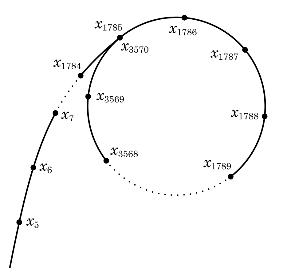
Pollard Rho

Pollard Rho is about finding collisions
A collision means two different steps → same point
It is useful because if aP + bQ = a'P + b'Q then (a − a')P = (b' − b)Q, which lets us solve for k
So the whole game is, “Walk randomly on the curve until you hit the same point twice” #Q How the random walk works ?
A We define a function f : G → G

• That means:
  • input: a point on the curve
  • output: another point on the curve
• We keep applying:

X₀
X₁ = f(X₀)
X₂ = f(X₁)
X₃ = f(X₂)
...

Sooner or later we will hit a point you’ve seen before

Q Why Pollard Rho is efficient ?
A when we consider naive attack we try k values which cost us “N” operations. where as in Pollard Rho we Find collision in about √N steps. And for finding this collisions pollard Rho uses “Two pointer method” This is why ECC key sizes must be large.

Applying Pollard Rho to Discrete Log (ECC case):
We want Q = kP

• Step 1: Split the group into 3 parts
  • We divide all points into: A, B, C (roughly equal size)
• Step 2: Define the function f
  • For a point X:
    • if X ∈ A → f(X) = X + P
    • if X ∈ B → f(X) = 2X
    • if X ∈ C → f(X) = X + Q
  • Why?
    • This gives good mixing (looks random)
    • Easy to compute
    • Easy to track coefficients
• Tracking coefficients: Every point X is stored as: X = αP + βQ
  • We track α and β at each step, for Example:
    • If X → X + P: then α increases by 1
    • If X → X + Q: then β increases by 1
    • If X → 2X: then α and β both double
  • So even though the walk looks random, we always know how X relates to P and Q.

Collision ⇒ solving for k:

• Suppose we find: Xᵢ = Xⱼ
• That means: αᵢP + βᵢQ = αⱼP + βⱼQ
• Rearranging: (αᵢ − αⱼ)P = (βⱼ − βᵢ)Q
• Since Q = kP, we get: k = (αᵢ − αⱼ) / (βⱼ − βᵢ) (mod N)
• As long as: gcd(βⱼ − βᵢ, N) = 1. we can compute the inverse and we can recover k

Pairings

A pairing is a special mathematical map that:

• Takes two elements from elliptic curve groups
• Outputs an element in a third group (usually multiplicative)
• In symbols:

$$e:G\times G\to G_T$$

• Where:
  • (G) is an additive group (elliptic curve points)
  • (G_T) is a multiplicative group (often a finite field)
  • Identity in (G): (0_G)
  • Identity in (G_T): (1)
• One thing to note is we write elliptic curve groups additively and we write the target group multiplicatively
• This is why:
  • (P + Q) is used in “G”
  • e(P, Q) multiplies in “G_T”

Properties of Pairing:

1. Non-Degeneracy
   • A pairing is non-degenerate if:

$$e(S,T)=1\forall S\in G\Rightarrow T=0_G$$

- If pairing output is always 1, then the map is useless. Such a map is called degenerate
- Non-degeneracy ensures:
    - Non-zero inputs give meaningful outputs
    - The pairing actually contains information

2. Bilinearity - The pairing is bilinear, meaning it is linear in both arguments - Linearity in the first argument:

$$e(S_1+S_2,T)=e(S_1,T)\cdot e(S_2,T)$$

- Linearity in the second argument:

$$e(S,T_1+T_2)=e(S,T_1)\cdot e(S,T_2)$$

3. Scalar Multiplication Property
   • From bilinearity, we get:

$$e([a]S,[b]T)=e(S,T{)}^{ab}$$

- Scalars in elliptic curves become exponents
- Allows algebraic manipulation across groups
- This property enables BLS signature, Signature aggregation and Identity-based cryptography

4. Alternating Property - A pairing is alternating if:

$$e(T,T)=1$$

- Pairing an element with itself gives identity
- Implies a form of symmetry restriction
- All pairings we use here satisfy this property

Weil Pairing

Every elliptic curve admits an efficiently computable pairing which is called the Weil pairing

• E be an elliptic curve
• E[m] be the (m)-torsion subgroup $$E[m]=P\in E\mid [m]P=0$$
• Then the Weil pairing is:

$$e_m:E[m]\times E[m]\to {\mu }_m$$

• Where:
  • u_m is the group of (m)-th roots of unity
  • Output lives in a multiplicative group

Degeneracy on Cyclic Subgroups:
In cryptography, we usually work in a cyclic subgroup which are generated by a point of large prime order but Unfortunately the Weil pairing is degenerate on such subgroups. This makes the raw Weil pairing not directly usable in practice
But this can be fix by introducing a distortion map:

$$\varphi :E\to E$$

Properties:

• It moves points outside the cyclic subgroup
• Preserves elliptic curve structure
• Not every curve admits such a map

Using a distortion map (\phi), we can define weil pairing as:

$$⟨P,Q⟩=e_m(P,\varphi (Q))$$

This pairing:

• Is non-degenerate on cyclic subgroups
• Preserves bilinearity and alternation
• Is suitable for cryptography
• This construction appears in early pairing-based crypto (e.g. Boneh)

BLS Signatures (Boneh-Lynn-Shacham)

• (G, G_T) be cyclic groups of prime order (p)
• (P) be a generator of (G)
• (e : G G → G_T) be a non-degenerate pairing
• (H : {0,1}^* → G) be a hash-to-curve function

Hash-to-curve:

• Maps messages to elliptic curve points
• Efficient and standardized in practice

Key Generation:

$$\text{Gen}(1^{\lambda }):$$

1. Sample: $$x\leftarrow {\mathbb{Z}}_p$$
2. Public key: $$pk:=[x]P$$
3. Secret key: $$sk:=x$$

Return:

$$(pk,sk)$$

Signing:

$$\text{Sign}(sk,m):$$

1. Hash message: $$Q\leftarrow H(m)$$
2. Compute signature: $$\sigma \leftarrow [x]Q$$

Return:

$$\sigma$$

• Signature is just one elliptic curve point

Verification:

$$\text{Verify}(pk,m,\sigma ):$$

Check:

$$e(\sigma ,P)\stackrel{?}{=}e(H(m),pk)$$

If true → accept
Else → reject

Q Why Verification Works ?
A Starting from the left:

$$e(\sigma ,P)=e([x]Q,P)$$

Using bilinearity:

$$=e(Q,P{)}^x$$

Rewriting:

$$=e(Q,[x]P)$$

Substitute (pk = [x]P):

$$=e(H(m),pk)$$

Aggregation Property:
Multiple signatures:

$${\sigma }_1,{\sigma }_2,\dots ,{\sigma }_n$$

Can be combined into:

$$\sigma =\sum _i{\sigma }_i$$

And verified once instead of (n) times

Summary:
Pairings:

• Connect elliptic curve groups to multiplicative groups
• Enable bilinear algebra
• Power advanced cryptography

BLS signatures:

• Are only possible because of pairings
• Are efficient, elegant, and modern
• Are actively used in real-world systems

Isogenies

Modern public-key cryptography relies heavily on problems such as Discrete logarithms, RSA (integer factorization) and Pairings on elliptic curves. However, All of these are broken by Shor’s algorithm on a sufficiently powerful quantum computer. This includes Classical ECC, RSA and Pairing-based cryptography
We can recover from this by switching to problems believed to be quantum-resistant. Main post-quantum families include Lattices, Codes, Multilinear maps and Isogenies
Here we focus on Isogenies
An isogeny is defined as A “nice” map between elliptic curves that respects both geometry (polynomial structure) and algebra (group law)
Elliptic curves are:

• Geometric objects (solutions to equations)
• Algebraic groups (points can be added)

Isogenies are special because they respect both views at the same time

Let E_1, E_2 be elliptic curves. An isogeny is a morphism (algebraic map):

$$\varphi :E_1\to E_2$$

such that:

• $\varphi (\infty )=\infty$ (the identity point maps to the identity point)
• phi is non-constant
• If such a map exists, we say E_1 and E_2 are isogenous

For example The curves

$$y^2=x^3+x\text{and}{y}^2=x^3-3x+3$$

are isogenous over F_17 via the map:

$$(x,y)\mapsto \left(\frac{x^3-4x^2+30x-12}{(x-2{)}^2},;y\cdot \frac{x^3-6x^2-14x+35}{(x-2{)}^3}\right)$$

This shows:

• Isogenies are rational functions
• They involve polynomials in numerator and denominator
• They map points to points on another curve

Properties of Isogenies:

1. Group Homomorphism
   • Every isogeny is also a group homomorphism:

$$\varphi (P+Q)=\varphi (P)+\varphi (Q)$$

- This means Point addition is preserved and the Algebraic structure is respected

2. Multiplication Maps are Isogenies - The map: [m]:E -> E (where a point is added to itself (m) times) is an isogeny - Reason: - Scalar multiplication can be written using polynomials - Identity maps to identity 3. Composition Works - We can compose isogenies:

$$E_1\stackrel{\varphi }{\to }{E}_2\stackrel{\psi }{\to }{E}_3$$

	and the result:

$$\psi \circ \varphi$$

	is still an isogeny
- This makes elliptic curves + isogenies a category (mathematically well-behaved)

4. Degree of an Isogeny - Each isogeny has a degree: - Measures how “large” or “complex” the map is - Can be defined as: - Size of the kernel - Degree of the defining rational functions - Multiplicativity If:

$$\varphi :E_1\to E_2,\psi :E_2\to E_3$$

	then:

$$\mathrm{deg}(\psi \circ \varphi )=\mathrm{deg}(\psi )\mathrm{deg}(\varphi )$$

5. Dual Isogeny
   • For every isogeny:

$$\varphi :E_1\to E_2$$

	there exists a unique dual isogeny:

$$\hat{\varphi }:E_2\to E_1$$

	such that:

$$\varphi \circ \hat{\varphi }=[\mathrm{deg}(\varphi )]$$

- It means
	- Go forward with `phi`
	- Come back with `\hat{\phi}`
	- Net effect = multiplication by the degree
- This is important as it allows isogeny graphs to be treated as undirected, which is crucial in cryptography

6. General Form of an Isogeny (Weierstrass Form) - Any isogeny between Weierstrass curves looks like:

$$(x,y)\mapsto \left(\frac{f(x)}{h(x{)}^2},;y\cdot \frac{g(x)}{h(x{)}^3}\right)$$

	- x-coordinate → rational function with square denominator
	- y-coordinate → multiplied by rational function with cube denominator
- This structure guarantees Curve equation remains valid and Group law is preserved

Separable and Inseparable Isogenies

Frobenius Isogeny:
Let:

$$E/k:y^2=x^3+ax+b\text{with }\text{char}(k)=p$$

Define:

$$E^{(p^r)}:y^2=x^3+a^{p^r}x+b^{p^r}$$

The map:

$$\pi :E\to E^{(p^r)},(x,y)\mapsto (x^{p^r},y^{p^r})$$

is called the p^r -Frobenius isogeny

There is a special case, it goes like
If:

$$k={\mathbb{F}}_{p^r}$$

then:

$$E^{(p^r)}=E$$

So Frobenius becomes an endomorphism of the curve

• Separable vs Inseparable
  • An isogeny is inseparable, if it factors through a Frobenius map
  • It is purely inseparable, if it is Frobenius followed by an isomorphism
  • Otherwise, it is separable
• We are mostly concerned with separable isogenies

Problems:
It is easy to find out if two curves are isogenous
Two curves E1 and E2 are finite field are isogenous over if and only if #E_1(k) = #E_2(k)
But finding isogeny is dramatically harder
The computational super singular isogeny problem is as follows: Given two super singular elliptic curves E, E’, find an isogeny between them, something like image below(we focus on second one)

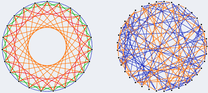
Isogeny Graphs:

• Let p, l be a primes, K a felid of characteristic p
• The l-Supersingular isogeny graph has as
  • Vertices: Supersingular elliptic curves over K
  • Edges: Separable isogenies from E -> E'
• Both up to isomorphisms(i.e.., vertices are j-invariants)
  • We can represent vertices as elements of (F_p)^2
  • Graph is directed
  • Graph has good mixing properties
  • Can walk in the graph with Velu’s method
  • Most vertices have degree l+1

Kernel and Velu

There is a one-to-one correspondence between Finite subgroups (H) of an elliptic curve (E), and Separable isogenies $\phi :E\to E^{\prime }$up to post-composition with isomorphisms In short Kernels <--> Separable Isogenies

• An isogeny is a morphism between elliptic curves that is also a group homomorphism
• Every isogeny has a kernel, which is a finite subgroup of the source curve
• This theorem says:
  • If you give me a finite subgroup H less than equal to E, I can construct an isogeny whose kernel is exactly H
  • Conversely, knowing the kernel completely characterizes the isogeny (up to isomorphism of the target)

The restriction to separable isogenies is essential; including inseparable ones breaks this clean correspondence

Vélu’s Formulas:
Let:

• E / k be an elliptic curve over a finite field k
• H less than equal to E a finite subgroup

Then:

• There exists an isogeny $\phi :E\to E/H$
• $\ker (\phi )=H$
• Vélu’s formulas allow us to compute:
  • The target curve (E/H)
  • The explicit isogeny map $\phi$
• Complexity: Theta(|H|)
• Vélu’s formulas give no control over the shape or quality of the target curve, only the kernel is guaranteed

Supersingular Curves

Let E / K with F_p
The curve (E) is Supersingular if:

• Multiplication-by-(p), [p] is purely inseparable
• $j(E)\in {\mathbb{F}}_{p^2}$ Otherwise, (E) is called ordinary
  Despite the name Supersingular curves are NOT singular but they’re perfectly smooth elliptic curves. The term refers to exceptional arithmetic behavior

Endomorphism Ring Characterization

For a Supersingular curve the endomorphism ring End(E) is an order in a quaternion algebra, This property does not hold for ordinary curves and is crucial for isogeny-based cryptography

Counting Supersingular Curves

Over (F_p)^n the #{supersingluar curves} = p/12 up to small constant adjustments depending on (p)

Number of Points

A Supersingular curve over F_P satisfies:

$$|E({\mathbb{F}}_p)|=p+1$$

This exactly matches the Hasse bound midpoint

This Super singular curves matter the most because Isogeny-based cryptography relies on walking in isogeny graphs and Supersingular graphs are Highly connected and Hard to navigate without secret kernels thus these are backbone of post-quantum isogeny cryptography

SIDH(Supersingular Isogeny Diffie-Hellman)

SIDH (Supersingular Isogeny Diffie-Hellman) is a key exchange protocol, like classical Diffie-Hellman, but built using elliptic curve isogenies instead of exponentiation
Its goal is simple “Allow two parties to agree on a shared secret over a public channel, even in the presence of a quantum computer”
Q Why SIDH exists ?
A Classical public-key systems rely on problems like:

• Discrete Logarithm (ECDH)
• Integer Factorization (RSA)

These are broken by quantum computers (Shor’s algorithm)
SIDH is based on a different hard problem which is “Finding an isogeny between two Supersingular elliptic curves”
The Core idea is SIDH replaces “raise a number to a secret power” with “walk secretly in a huge graph of elliptic curves”
SIDH works with:

1. Supersingular elliptic curves
2. Isogenies (special maps between elliptic curves)
3. Isogeny graphs
   • Nodes = elliptic curves
   • Edges = small-degree isogenies

Classical DH	SIDH
Public base (g)	Public starting curve (E)
Secret exponent	Secret isogeny
(g^a), (g^b)	Public curves after secret walks
(g^{ab})	Shared curve

Working of SIDH

• Step 1: Public setup
  • Everyone agrees on:
    • A large prime (p)
    • A Supersingular curve E / (F_P)^2
    • Some public torsion points
  • This is like choosing (g) in Diffie-Hellman
• Step 2: Secret choices
  • Alice chooses a secret isogeny of degree 2^{e_A}
  • Bob chooses a secret isogeny of degree 3^{e_B}
  • These correspond to hidden paths in different parts of the isogeny graph
• Step 3: Public keys
  • Alice publishes the curve she reaches
  • Bob publishes the curve he reaches
  • Plus some extra information (torsion point images)
  • This is like publishing g^a andg^b
• Step 4: Shared secret
  • Alice continues Bob’s walk using her secret
  • Bob continues Alice’s walk using his secret
  • Both end on isomorphic curves
  • The shared secret is j-invariant of final curve

Q Why it works ?
A Isogenies commute up to isomorphism

$$E/⟨A,B⟩\cong E/⟨B,A⟩$$

So even though:

• Alice goes “right then down”
• Bob goes “down then right”

They land at the same final curve

Q What makes SIDH hard to break ?
A An attacker sees starting curve, public curves, and torsion point images. But does not know secret kernels and secret paths in the graph
Recovering them requires solving the “Computational Supersingular Isogeny Problem (CSSI)”

• SIDH itself is broken (due to active attacks)
• SIKE, a variant using transformations, was also broken in 2022
• But the math and ideas are still important and foundational

SIKE(Supersingular Isogeny Key Encapsulation)

SIKE (Supersingular Isogeny Key Encapsulation) is a CCA-secure construction built on top of SIDH. It exists because SIDH by itself is not secure against active attacks and SIKE fixes this by applying the Fujisaki-Okamoto (FO) transform

Properties:

• Very short key sizes compared to other PQ schemes
• Slower than lattice-based schemes
• Best known attacks are classical, not quantum

Fujisaki-Okamoto (FO) transform

The Fujisaki–Okamoto (FO) transform is a generic cryptographic technique used to convert a public-key encryption (or key exchange) scheme that is secure against passive attacks into one that is secure against active (chosen-ciphertext) attacks
In short “FO transform upgrades IND-CPA security → IND-CCA security”

Algorithm:
The FO transform binds randomness, message, and ciphertext together using hash functions, so that Any modification of the ciphertext or incorrect decryption results in random, useless output
Assume we have:

• A public-key encryption scheme Enc(pk, m; r) and Dec(sk, c)
• Cryptographic hash functions H, G

Encryption (Encapsulation):

1. Pick random value m
2. Derive randomness: r = H(m, pk)
3. Encrypt using deterministic randomness: c = Enc(pk, m; r)
4. Derive shared key: K = G(m, c)
5. Output: Ciphertext c and Shared key K

Decryption (Decapsulation)

1. Decrypt ciphertext: m' = Dec(sk, c)
2. Recompute randomness: r' = H(m', pk)
3. Re-encrypt: c' = Enc(pk, m'; r')
4. Check:
   • If c' ≠ c → output random key
   • Else → output G(m', c)

Q Why This Works (Intuition) #A

• An attacker cannot forge valid ciphertexts without knowing m
• Any tampering causes the ciphertext check to fail
• Failed checks leak no information
• Replay and malleability attacks are neutralized

Security

There is an underlying hard problem that is the security is based on the CSSI problem “Computational Supersingular Isogeny problem”

Q Given two Supersingular elliptic curves E_0 -> E_1 over F_{p^2}. Find an ℓᵃ-isogeny between them ?
A Attack strategy described

• Let k = a/2

• Define sets of cyclic subgroups:

  $$S_{i,k}:=H\le E_i[{\ell }^k]\mid H\text{ cyclic},|H|={\ell }^k$$

• Define:

  $$S:=(0\times S_{0,k})\cup (1\times S_{1,k})$$

• Define function:

  $$g:S\to {\mathbb{F}}_{p^2},(i,H)\mapsto j(E_i/H)$$

• A collision: g(0,H) = g(1,H'), this solves the CSSI problem

Q what’s the solution for Pollard-Rho style attack ?
A

• Use a hash function: $$h:{\mathbb{F}}_{p^2}\to S$$
• Define iteration: $$f:=h\circ g$$

This enables collision-finding attacks

van Oorschot–Wiener (vOW) algorithm:

• Hash maps a set of size ≈ p/12 to a set of size ≈ p¹ᐟ⁴
• This introduces many collisions
• vOW algorithm is used to find the “golden collision”
• Time complexity is O(p^{3/8})
• This is the best known classical attack

Summary

Elliptic Curve Cryptography (ECC) starts from number theory (Diophantine equations), builds a group structure on elliptic curves, uses hard problems like the discrete logarithm for security, enhances capabilities using pairings, and finally moves to isogenies and Supersingular curves to design post-quantum cryptography (SIDH/SIKE). Classical ECC relies on DLP hardness; post-quantum ECC relies on hardness of finding isogenies between Supersingular curves

1. Diophantine Equations
   • Equations with integer or rational solutions
   • Elliptic curves arose from studying equations like:
   $$y^2=x^3+ax+b$$
   • What began as pure mathematics became cryptography
   • Why it matters: Elliptic curves originate from number theory, not crypto design
2. Mathematical Background
   • Covers:
     • Modular arithmetic
     • Finite fields F_p and F_{p^k}
     • Groups, rings, fields
     • Why it matters: ECC lives entirely inside finite fields and group theory
3. Elliptic Curve Definitions
   • An elliptic curve over a field (K): E: y^2 = x^3 + ax + b
   • with non-singularity condition: 4a^3 + 27b^2 != 0
   • Why it matters: Defines the object on which cryptography is built
4. Discriminant

$$\Delta =-16(4a^3+27b^2)$$

- `Delta != 0` ⇒ curve is smooth
- `Delta = 0` ⇒ curve is singular (invalid)
- Why it matters: Guarantees a well-defined group law

5. j-Invariant

$$j(E)=1728\frac{4a^3}{4a^3+27b^2}$$

- Classifies elliptic curves up to isomorphism    
- Same (j) ⇒ same curve shape
- Why it matters: Isogeny-based cryptography works by hiding j-invariants.

6. Representation and Group Law - Elliptic curve points form an abelian group: - Point addition via geometry - Identity: point at infinity “O” - Why it matters: Cryptography needs groups with efficient operations 7. Scalar Multiplication

$$[k]P=P+P+\cdots +P$$

- Core operation in ECC
- Efficient via double-and-add
- Why it matters: ECC security = easy forward, hard reverse

8. Number of Points on an Elliptic Curve - Hasse’s theorem:

$$|E({\mathbb{F}}_p)-(p+1)|\le 2\sqrt{p}$$

- Why it matters: Group size determines security level

9. Discrete Logarithm Problem (DLP) - Given: P, Q = [k]P
- Find (k) - Why it matters: ECC security rests on DLP being hard 10. Pollard Rho - Best classical algorithm for ECC DLP - Time Complexity: O(√n) - Why it matters: Defines real security bounds for ECC 11. Pairings - Maps: e: G_1 x G_2 -> G_T - Converts group problems into field problems - Why it matters: Enables advanced crypto primitives 12. Weil Pairing - Concrete bilinear pairing on elliptic curves - Efficient and non-degenerate - Why it matters: Foundation for pairing-based cryptography 13. BLS Signatures - Uses pairings to allow Very short signatures and Signature aggregation - Why it matters: Modern blockchain and distributed systems rely on this 14. Isogenies - Structure-preserving maps between elliptic curves - Group homomorphisms + algebraic maps - Why it matters: Isogenies are hard to reverse, even with quantum computers 15. Kernel and Vélu - Every separable isogeny ↔ finite kernel - Vélu’s formulas construct isogenies from kernels - Why it matters: Practical computation of isogenies 16. Supersingular Curves - Special elliptic curves with Huge endomorphism rings and Exceptional symmetry - Why it matters: Only supersingular curves give hard isogeny problems 17. SIDH (Supersingular Isogeny Diffie-Hellman) - Diffie-Hellman analog using isogenies - Keys = secret kernels - Exchange j-invariants - Why it matters: Post-quantum key exchange candidate 18. SIKE (Supersingular Isogeny Key Encapsulation) - SIDH + Fujisaki-Okamoto transform - CCA-secure KEM - Why it matters: Attempts to make SIDH safe in real networks (historically important despite later breaks) 19. Security - Classical ECC → broken by Shor - Isogeny crypto → quantum-resistant - Security relies on CSSI (Computational Supersingular Isogeny problem)